Overview
In this project, I was able to take what I learned from lectures and implement them into actual code. First, I started from the basics, simply working on rasterizing single-color triangles, before moving on to more advanced techniques, such as supersampling to reduce aliasing effects. Then, I worked on creating simple transform functions, using them to do things such as translating and scaling an image, before developing a system for barycentric coordinates that helped create smoothly blended color triangles. Lastly, I implemented different methods of sampling in order to fine tune an image, allowing for texture mapping.
Overall, I think it was amazing how the project turned out as a whole! It was really satisfying being able to fine tune and tweak the images that I produced, and to witness visually the effects of the work that I put in. Some things that I learned are to be careful of integer overflow when sampling, since its possible to get invalid x and y values as you zoom into an image, as well as that although there seems to be an extremely large amount of computation going into the rendering of these images, even seemingly small design choices can have a large impact on efficiency. For example, just putting a bounding box around each triangle that we attempt to rasterize shaves off a significant amount of time and effort.
Section I: Rasterization
Part 1: Rasterizing single-color triangles
As a general overview of rasterization, the process involves turning a description of an image into its pixel form. Specifically, rasterizing triangles is the method of taking the triangles that compose an image and converting them into pixels of color, depending on whether or not they are within the boundaries of the triangle. Essentially, we start off with the coordinates of three different points, that when connected form the boundaries of a triangle. In order to rasterize it, we look at corresponding pixels in our grid to determine if it is inside or outside the triangle; if inside, we choose to color that pixel with the specified color.
My original naive algorithm, in order to test the general process, was to iterate through all possible pixels within the image, and check if the center of the pixel was within the boundaries of the triangle. I defined a helper function that returned the float value of plugging in the given point into the line equation between two points of a triangle, and then used it in another helper function to check if the pixel center was on exactly the same side between each test. If so, then the helper function returned that the pixel center was in fact within the boundaries of the triangle. From there, it was a simple matter to simply fill the chosen pixel in, by calling the fill_pixel function.
For the sake of efficiency, instead of iterating through all the pixels in the image, I only iterated through pixels within the boundary box (i.e.: in the horizontal direction, from the lowest to highest x value, and in the vertical direction, from the lowest to highest y value). Everything not within the bounding box is guaranteed to not be in the triangle anyway, so it makes sense to only check specifically for those pixels. I also tried adding some tolerance to the range, and experimented with adding anywhere from 1 to 10 additional pixels within the ranges, but I didn't actually notice any real effect from doing so.
Here is an example of the basic algorithm at work! Notice that in parts of the triangle where there is a very sharp edge, the corner actually appears to be disconnected from the rest of the triangle. This is due to the strict way in which we sample and assign a color to each pixel, which can be fixed in the future using other sampling methods.
|
Part 2: Antialiasing triangles
While standard rasterization techniques with triangles works relatively well, they still produce some unwanted aliasing effects, such as jaggies or disconnections throughout the image. One such example is the above figure, where the top corner of the pink triangle actually gets disconnected from the rest of the body! In order to avoid this, I implemented supersampling, which essentially splits an individual pixel into a chosen number of parts, and checks whether each of those subpixels are inside the triangle; then, the pixel is assigned the average of all the colors of its subpixels.
In order to implement supersampling, the first thing was needed was an additional buffer supersample_buffer that could be used to store the color values of all the individual subpixels. While the original rgb_framebuffer_target was only the size of the area of the actual image, the supersample_buffer had enough space to account for each subpixel throughout the image. Then, most of the implementation details went into making every function work with this new buffer, whether I needed to clear the buffers, change the sampling rate, width, or height of the image, or change the current image on the screen.
Additionally, I needed to fix my rasterization function for triangles such that it iterated through individual subpixels based on the current sampling rate. This was done with some quick calculations of the number of pixels in each row and column and then stepping into one subpixel at a time. I also made sure to use the center of each subpixel as the reference point for that pixel, in order to determine if it was inside the given triangle. Additionally, I kept a sample_counter to help keep track of indexing into my supersample_buffer, where each given subpixel could be inserted into the buffer through the index (s * width * height) + (width * y) + x.
Lastly, I needed to account for the conversion from the supersample_buffer to the rgb_framebuffer_target. To do this properly, I iterated through each pixel in the image, and appropriately indexed into the supersample_buffer using the previously described index scheme to get the colors of each of its subpixels. I then averaged all of those colors together, and assigned the new color to the main pixel in rgb_framebuffer_target.
Here is an example of the benefits of the supersampling! Below are the same test image as before, this time sampled at different rates in order to protect against aliasing. Notice how the previously detatched corner seems to join back with the main body as the pixels begin to average together.
|
|
|
|
|
One additional thing I noticed here after I had worked a little further into the project, was that when I zoomed in on the images too much, the program would crash. After some experimentation with the debugger, I realized that due to integer overflow, some of the x and y values were going out of bounds as I zoomed into the screen. A simple bounds check before actually sampling the subpixel helped to alleviate this problem.
Part 3: Transforms
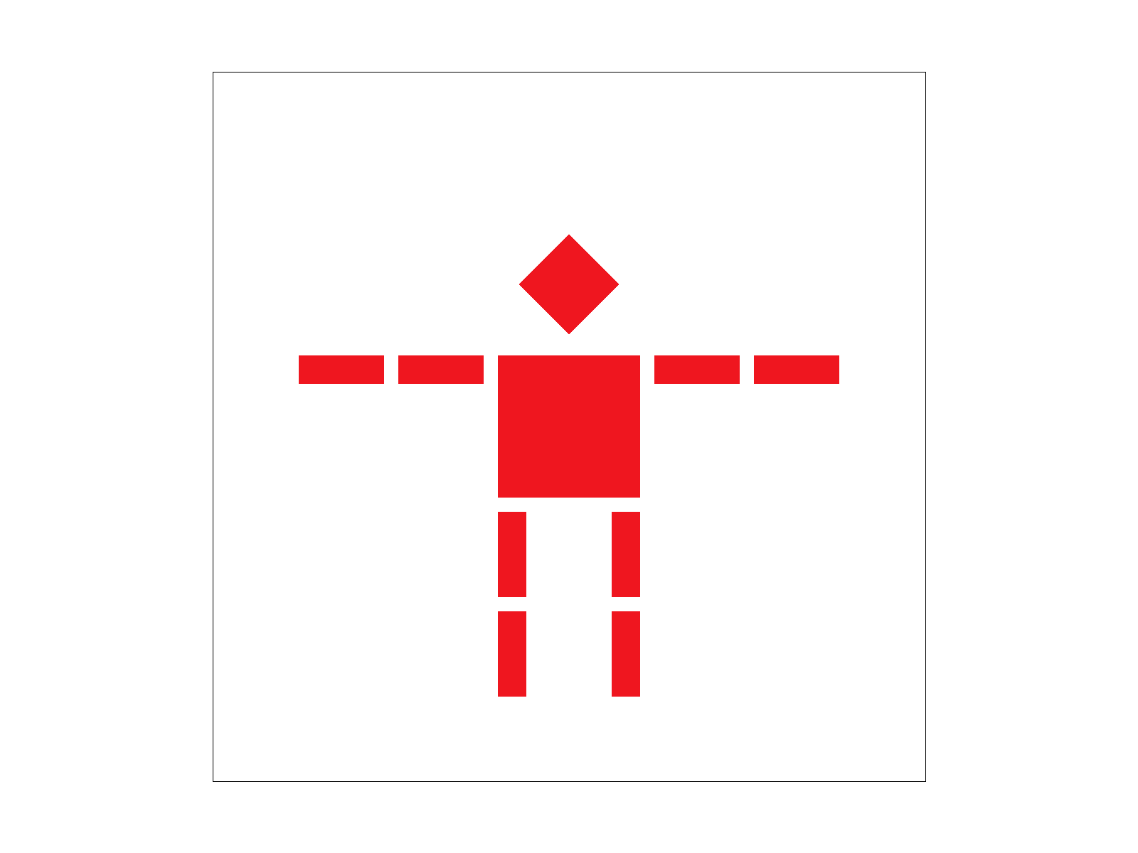
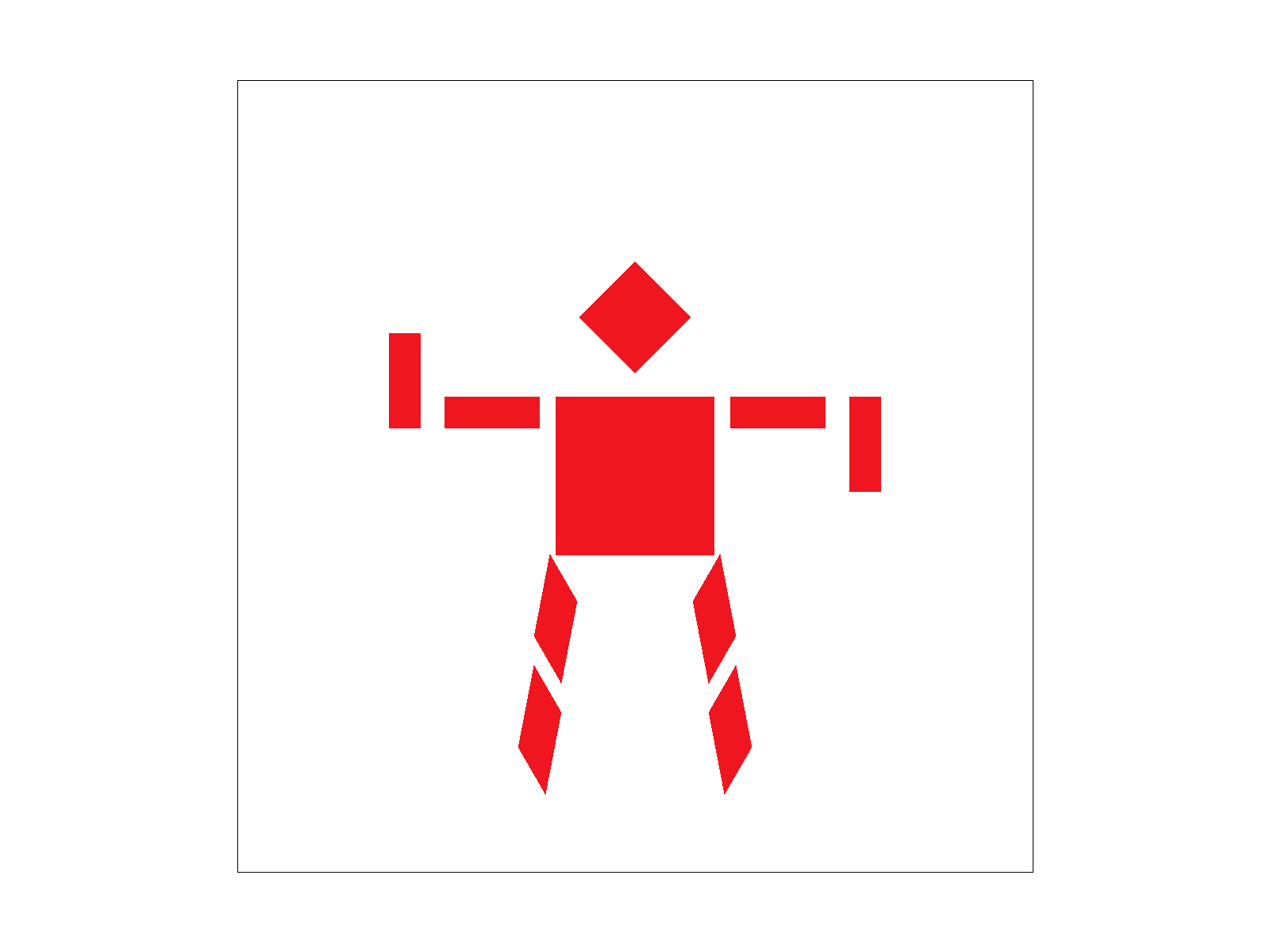
Here I implemented the three transforms of scaling, rotating, and translating, as described in lecture. I could then use these transformations to affect the position and actions of this robot! Below is a comparison between the original robot's position versus how I made him transform. In order to do this, I had to rotate the left and right hands by 90 degrees first, and then edited the translation of the arms so they fit nicely next to the robot's arms. I also rotated the legs of the robot by 30 and -30 degrees for the left and right legs respectively, in order to get this open legged effect.
|
|
All of these transforms are implemented using simple matrix multiplication in homogenous coordinates. Converting into these coordinates allowed for various transformations such as translations to be expressed as a linear operator when they previously were not.
Section II: Sampling
Part 4: Barycentric coordinates
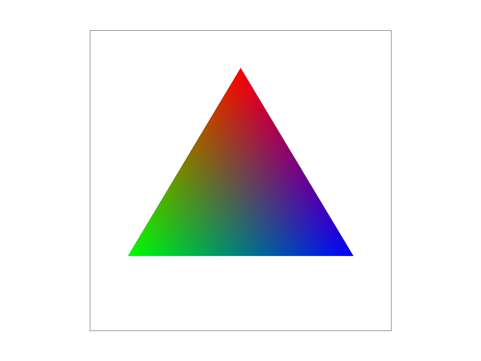
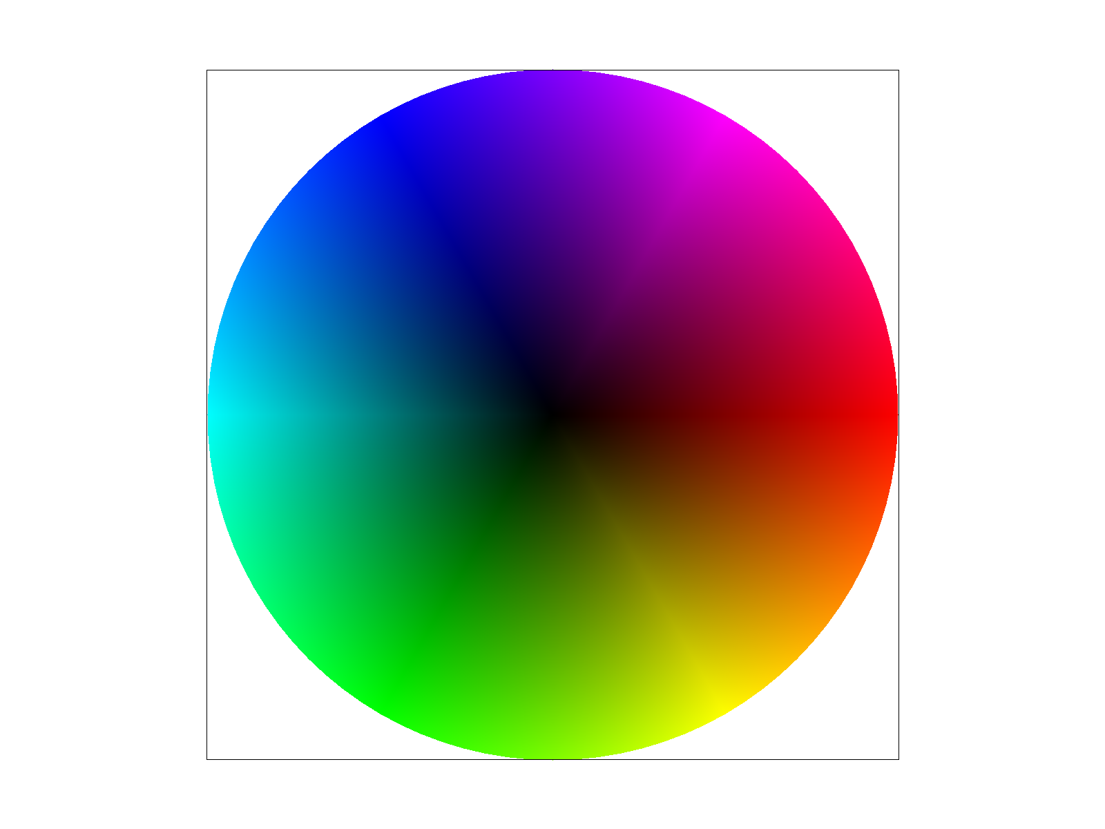
The idea behind Barycentric coordinates is that if we have colors associated with vertices of a triangle, then we can assign colors to points inside the triangle based on their proportional distance to each of the given vertices. These proportions can be given as some alpha, beta, and gamma, and their sum has to equal one. For example, this can be demonstrated by the following triangle, where each vertex corresponds to either red, green, or blue. The exact center of this triangle would result in an (almost) equal distribution of all three of those colors. The way the colors blend together all through the inside of the triangle is a result of that proportional distance. In addition, the color wheel is also representative of that same Barycentric coordinate system.
|
|
Part 5: "Pixel sampling" for texture mapping
The idea behind pixel sampling for texture mapping is that given a surface point, we want to be able to map it to its corresponding texture coordinate (texel), so that we can apply a specific texture to the selected pixel. The conversion into texture space allows us to visualize texture coordinates in a flat grid, with (u, v) coordinates, take our pixel and map it to that grid, find the appropriate color sample, and then apply it to the pixel in the normal image space. We do this using barycentric coordinates, and calculate the texture value for each sample.
Since there is usually not a strict one-to-one mapping between pixel and texel, it was necessary to look into different pixel sampling methods that helped to alleviate this. The first one that I implemented, nearest-pixel sampling, looks at the closest texel to the (u, v) coordinate of the converted pixel and uses that as its color choice. The second one, bilinear sampling, takes the (u, v) coordinates of the pixel and finds the four closest texels relative to that pixel. It then linearly interpolates with the pixel horizontally and vertically to find the appropriate color matching.
Below are the same image using nearest-pixel and bilinear sampling, with sample rates of 1 and 16 respectively. Notice that while nearest-pixel has more artifacts when using the texture mapping, bilnear sampling attempts to smoothen it out, although it doesn't completely fix the problems. This can be alleviated through the use of supersampling, although it is very computationally expensive for a large image.
|
|
|

|
|
The two methods will have very different results from each other if the pixels do not have a very unique mapping to their texels. For example, if it is very ambiguous if a pixel should map to a specific texel, nearest-sampling will just select a texel and be done with it, whereas bilinear sampling will interpolate the closest colors to find the best combination. This means in general, bilinear sampling will be smoother, although it can definitely depend on the image in question.
Part 6: "Level sampling" with mipmaps for texture mapping
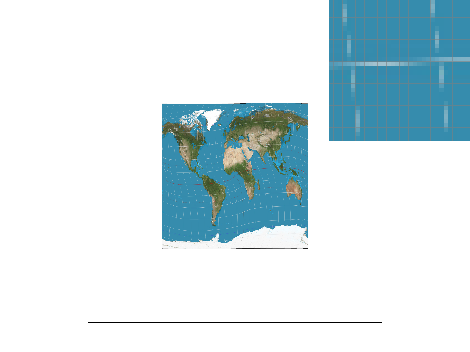
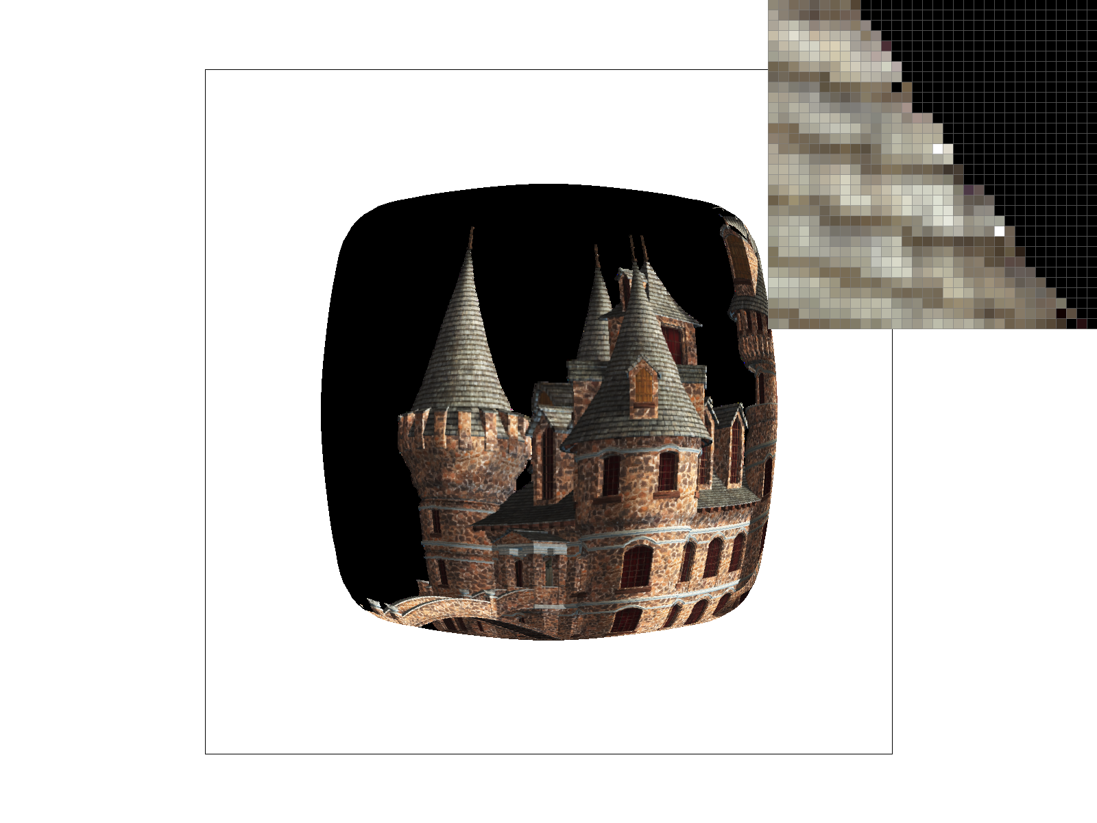
The idea behind level sampling is that we can store different downsampled textures of our image in a mipmap, so that if we have multiple perspectives in an image, we can render their textures separately from each other. The classic example of this is a castle, where the bricks that are close are rendered clearly, while those that are far are more blurred out. We can then select the appropriate level in the mipmap in order to render the texture as desired.
Based on the spec, I implemented three different level sampling methods. The first one L_ZERO, was simple and only used the 0-th level of the mipmap. The second one L_NEAREST, used the closest level in the mipmap as calculated by the rounded maximum of the norms of the partial derivatives of the uv coordinates with respect to x and y. The last one L_LINEAR used the same function to find the position of the closest level, and then calculate the closest two adjacent levels to interpolate between them and find the appropriate texture, with a ratio based on the position in between.
There are certain tradeoffs between the combinations of each of the pixel and level sampling methods. Nearest pixel sampling is quick and computationally easy, although the fact that it just takes the closest texel means that it is more prone to aliasing and a more jaggie-filled image. This is in comparison to bilinear sampling, where it is definitely much more computationally taxing to compute the interpolation between the four colors, but it will definitely give a smoother image when the pixels aren't neatly associated with a given texel. For level sampling, only using level 0 will use less memory overall, will be faster, but will not prevent aliasing at all. Between the nearest level and using the combination of the two adjacent levels, the nearest level option will require less memory than using multiple mipmap levels, but will have a worse antialiasing effect compared to the continuous version. Additionally, the continuous linear version will use slightly more computation to interpolate between the two given levels.
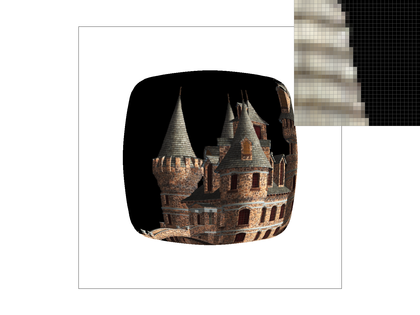
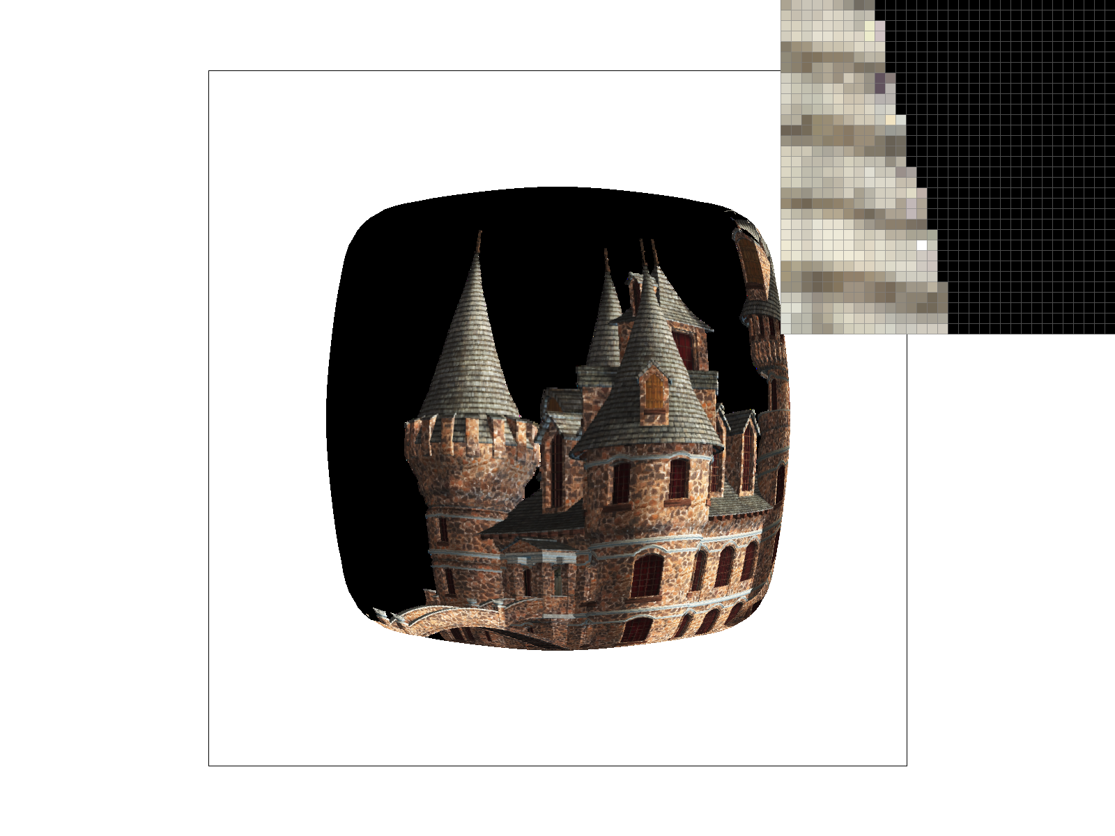
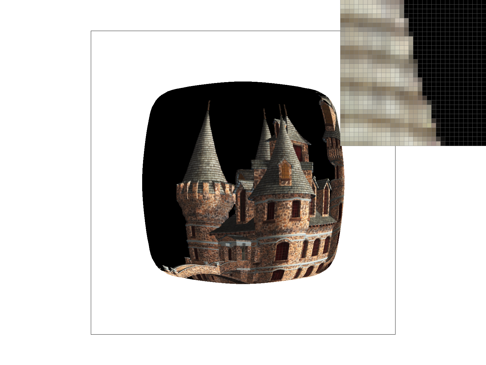
Below are different combinations of L_ZERO, L_NEAREST, P_NEAREST, and P_LINEAR. Notice that the difference between pixel sampling is pretty distinct, as going from nearest to linear really smoothens out the picture. We can also see how the distance between mipmap levels affects the visualization, where it becomes smoother and more textured at further distances.
|
|
|
|