Part 1: Ray Generation and Intersection

Task 1: Generating Pixel Samples

In order to begin working on my implementation to ray trace pixels, I needed to generate rays at different positions within the given pixel. For this, I first uniformly sampled an x and a y from [0,1], and then added that offset to the bottom left corner of the pixel. This would give a new location at a position somewhere within the pixel. I then called the generate_ray function at that position normalized in order to get a ray through that position. From there, I estimated the scene radiance along that ray using the est_radiance_global_illumination(...) function, to get a Spectrum value of the pixel. For any given pixel, I did this ns_aa times, before just averaging all the results together and then updating the specific pixel with that value.

Task 2: Generating Camera Rays

To generate the camera rays, both the origin and direction, I needed to convert the normalized position inputted from image space to camera space. To do this, I multiplied each input correspondingly by tan(radians(0.5 * Fov)), where each Fov is either the horizontal or vertical field of view depending on which component is getting multiplied. Then, I multiplied this position with the c2w matrix, converting the camera space coordinates into world space, before then normalizing this vector to get a direction. For the origin, I just used the provided pos as the origin of the camera in world space. I also initialized the min_t and max_t of the ray as nclip and fclip, the near and far clipping planes, making sure to only consider values within this range as visible to the camera.

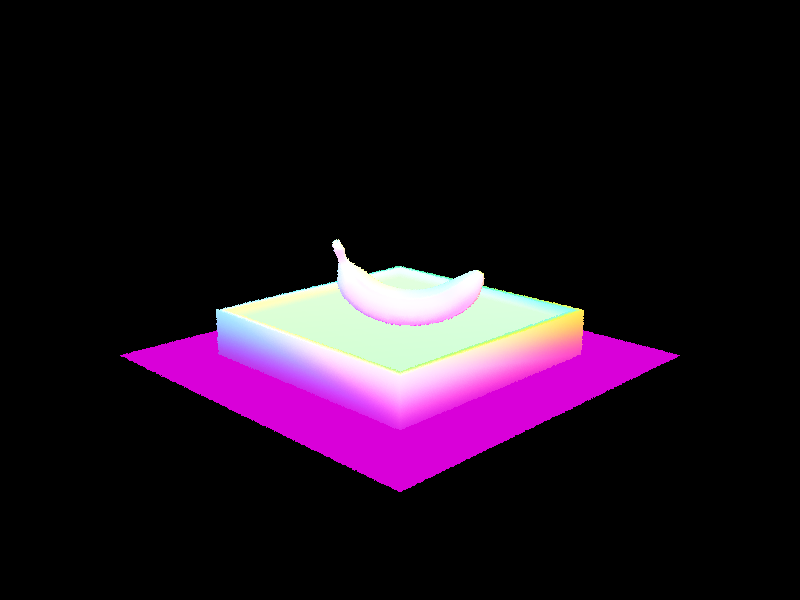
Completing these two tasks allowed me to generate the following images before moving on to testing for intersections:

Task 3: Ray-Triangle Intersection

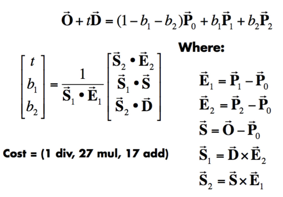
In order to efficiently compute ray-triangle intersections, I made use of the Moller Trumbore Algorithm, listed here, taken from the lecture slides:

Moller Trumbore is derived using Cramer's Rule using determinants and minimal computations in order to compute the intersection point. For the algorithm, I put in the points within the triangle as P0, P1, and P2, as well as the origin and direction of the ray itself, to compute all the necessary vectors using cross and dot products to produce the resulting vector of t, b1, and b2.

From this procedure, I got that t was the value at which the ray intersects the triangle, and b1 and b2 were Barycentric coordinates. Based on whether the t was correctly within the range of min_t and max_t of the ray, and all the Barycentric coordinates were between 0 and 1, I updated the intersection of the ray and the triangle appropriately, while also updating the max_t of the ray. To do this, I used the Barycentric coordinates I just computed, b1, b2, and 1-b1-b2, in order to compute the surface normal of the triangle based on the normals at each of its vertex points. I also updated the primitive attribute to be 'this' and the bsdf attribute to be the result of calling get_bsdf().

The following is the result of rendering the same scene as before after being able to compute the intersection between rays and triangles:

Task 4: Ray-Sphere Intersection

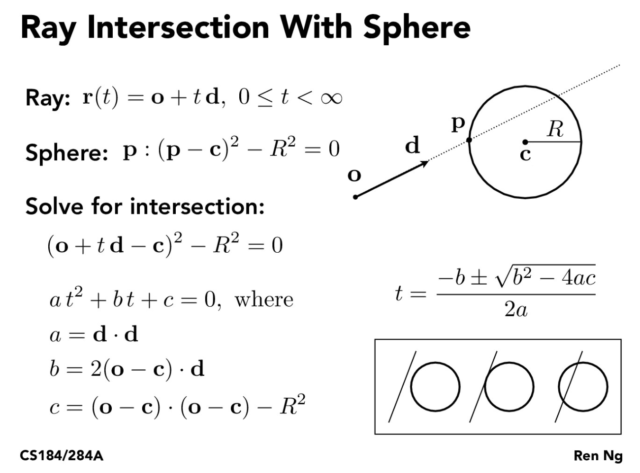
The last part of this task was to be able to detect and find ray-sphere intersections. To do this, I made use of the following slide, using the general equation of the sphere and the equation of the ray to compute the two intersection points:

By plugging the ray equation into the sphere equation, I can then use the quadratic formula to solve for the values of t, which can be updated for the intersection accordingly. This time, in order to check for valid intersections, I looked at the value of the discriminant, b^2 - 4ac. If the discriminant is positive, the ray intersects the sphere at exactly two points, and I can find those t values by solving the quadratic equation normally. If the discriminant is negative, the ray does not intersect the sphere, and I ignore the current results. If the discriminant is zero, the ray perfectly intersects the sphere at exactly one point, and I compute the same t value for both the minimum and maximum. I can then update the min_t and the max_t of the ray to be the smaller and larger of the two intersection t values respectively, and then update the normal to be the vector from the center of the sphere to the first intersection point.

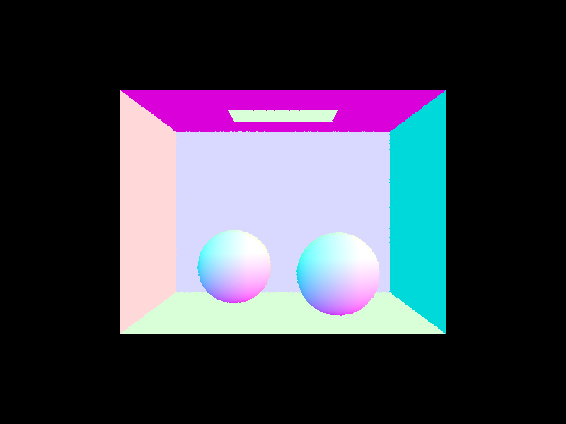
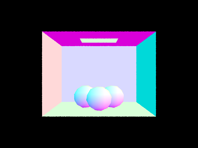
Below are the results of various renderings after implementing the ray-sphere intersections:

Part 2: Bounding Volume Hierarchy

Task 1: Constructing the BVH

Even though I could now render using ray-tracing with triangle and sphere intersections, certain renderings were just much too slow to get done in a sizable amount of time. To combat this, I created a Bounding Volume Hierarachy (BVH) to essentially prevent needless intersection checks between rays and primitives. I used a recursive algorithm in order to construct the BVH, where I partitioned objects into either a left or right child node based on their relationship with the average centroid of all the objects at the current node. Then I implemented a base case that said upon reaching a point where there are less than or equal to max_leaf_size number of objects, I grouped those objects into that node, creating an iterator through the list of objects and saving it to that node. Choosing the splitting point between left and right child nodes was a little tricky, but I eventually settled on first finding the axis of most variance between the x, y, and z of the bounding box, and then using the specific value at the average centroid of all the objects at the current node along that axis as the midpoint. From this, I was able to easily sort objects into either a left or right side with ease. In the specific edge case where all objects were sorted into just one side, I decided to just consider that to be a leaf node instead of further splitting. Additionally, each node had its own bounding box that was relative to its individual objects that were assigned to it.

Task 2: Intersecting the Bounding Box

From here, I defined the function BBox::intersect(...), which would allow me to determine whether a ray intersected the bounding box of the current node. I took the minimum and maximum corners of the bounding box, and then used the formula min / max = (1.0. / ray_direction) * (min / max - ray_origin) to get various t values of intersection for each axis. Then, I took the maximum over the minimums to get the min_t of intersection, and the minimum over the maximums to get the max_t of intersection. From here, I just used those values of t to determine if the ray validly intersected the bounding box, with the criteria that min_t had to be less than max_t, and the range of the ray's min and max t should intersect with the bounding box's. The function did this with some boolean logic, and then returned whether the ray actually intersected the box.

Task 3: Intersecting the BVH

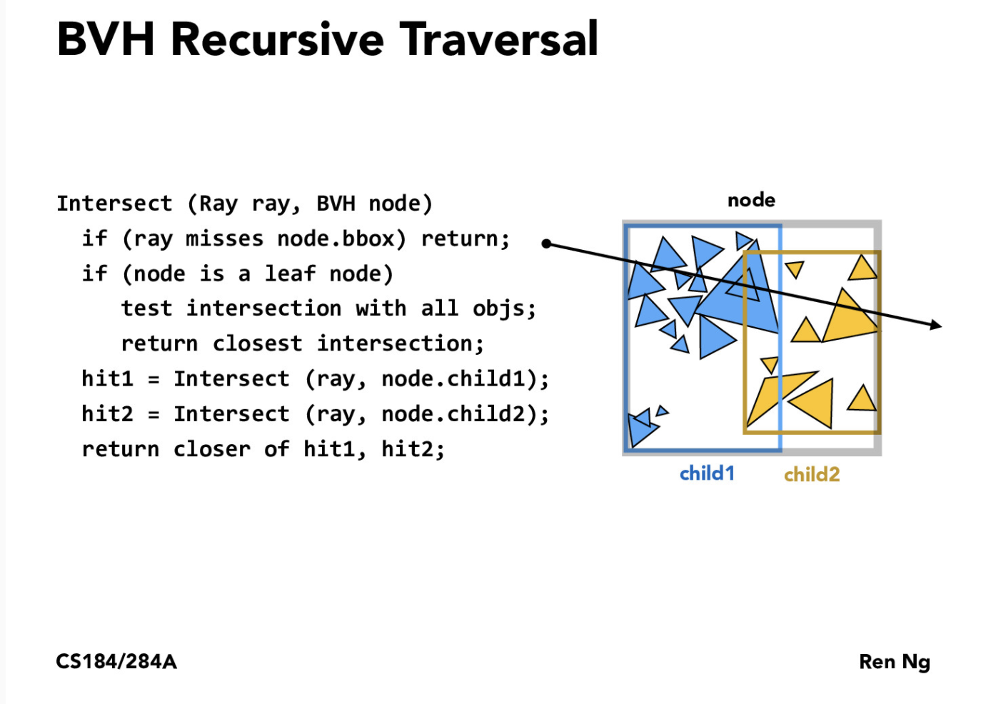
Finally, to use the BVH, I implemented the following pseudocode in the intersect(...) function, taken from lecture slides, in order to traverse the BVH recursively:

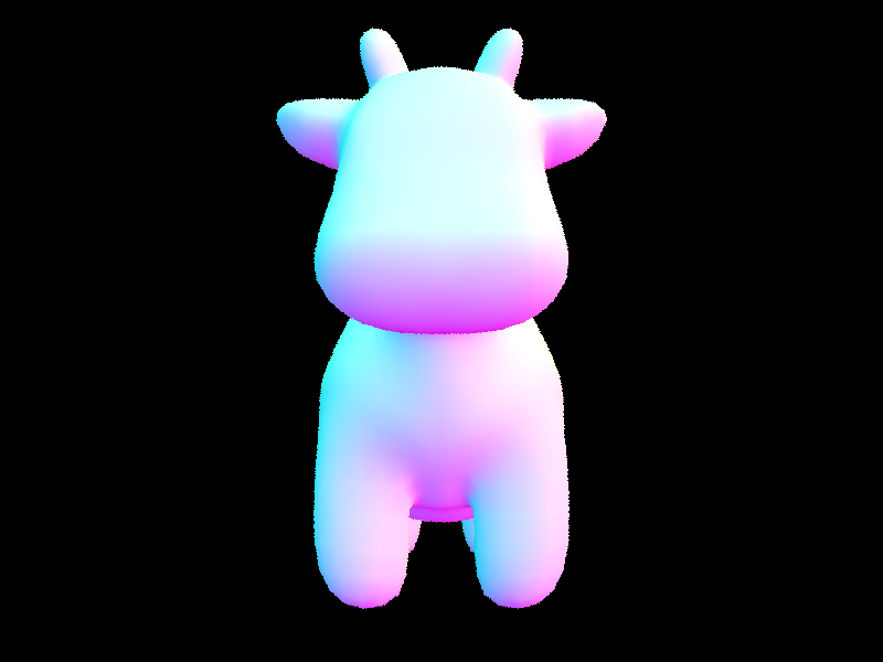
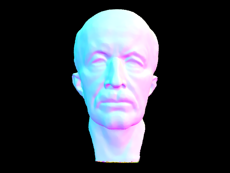
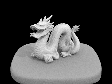
Essentially, I check whether the ray intersects the current bounding box, before then checking for intersection with its children nodes. Upon reaching a leaf node, I individually check each primitive object within the bounding box for intersection. I also implemented a has_intersection(...) function which just determined whether the ray intersected any object at all, whereas the intersect(...) function searched for the nearest point of intersection. By recursively moving through the BVH and making sure to only check intersections within primitives that were in bounding boxes that the ray intersected, I was able to save a significant amount of computation time, going from and O(n) to O(log(n)) runtime. Below are some examples that I was able to render using this significantly faster method:

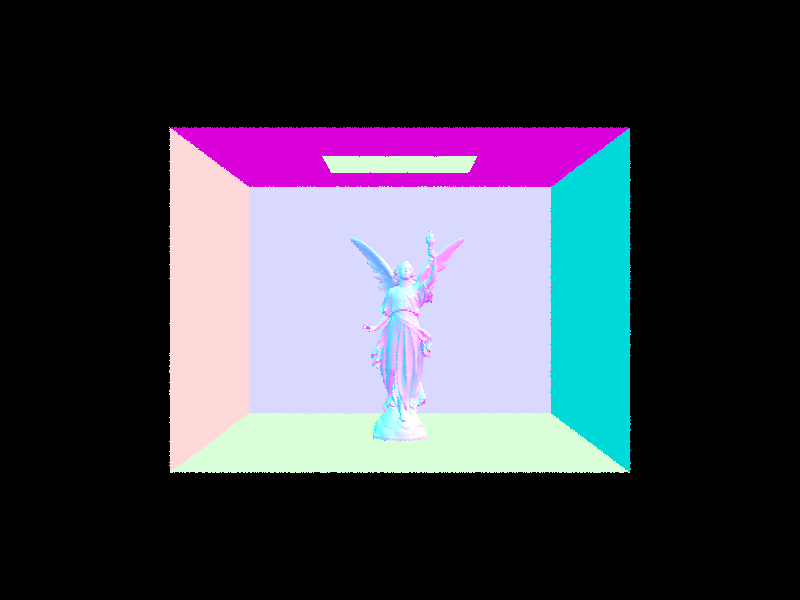
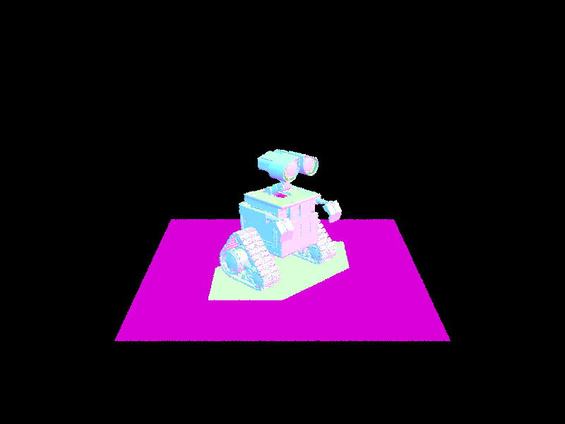
Comparing the runtimes with and without BVH, the cow took approximately 30 seconds to render without BVH on my local machine, while with BVH, it rendered in only .0466 seconds! Additionally, those with complex geometries such as CBlucy and Wall-E weren't even anywhere close to rendering after several minutes without BVH, but managed to render in 0.0551 and 0.0848 seconds respectfully once I implemented the BVH. Essentially, even doubling or tripling the number of triangles in the model did not significantly increase the runtime, and the use of the BVH to ignore a significant amount of computation meant that complex models could be rendered that previously couldn't have been before! Mathematically this runtime with the use of the BVH can be written as O(log(n)), with n being the number of triangles in the scene.

Part 3: Direct Illumination

Task 1: Diffuse BSDF

Material properties can be quantified using the BSDF of the material. For this part, I implemented the f and sample_f functions for a diffuse BDSF material, which is just a constant since diffuse material reflects light equally over all directions. As a result, the functions both just returned the reflectance of the material divided by pi, and so the proportion of incoming light scattered from the incoming light ray wi to the outgoing light ray wo did not actually depend on the input rays.

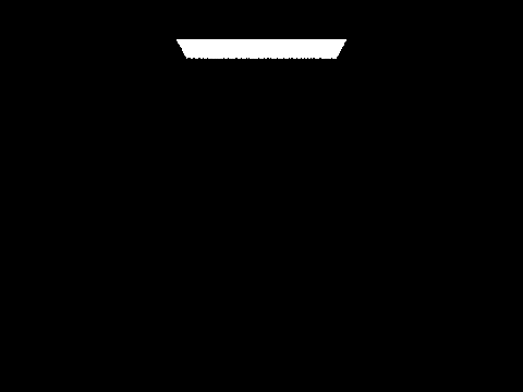
Task 2: Zero-bounce Illumination

As a general sanity check, I implemented zero-bounce illumination, just rendering light without implementing any bounces. Basically, I created a function that directly returns the emission of the object when intersected. As a result, only light sources would be visible in the scene. As a demonstration, this is the result of rendering a 3D bunny scene with zero-bounce illumination. Notice that nothing is actually visible except for the light source itself on the top:

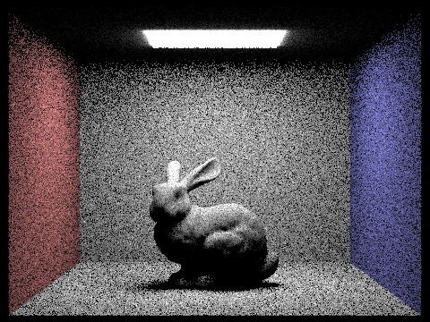
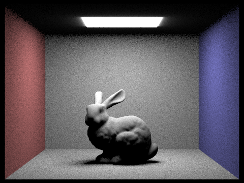
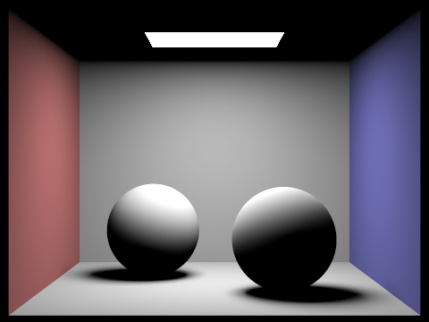
Task 3: Direct Lighting with Uniform Hemisphere Sampling

In order to actually render objects with lighting, I first attempted to do it by uniformly sampling the hemisphere! Essentially, I first defined hit_p, the hit point of the input ray onto the object, and w_out, the vector in world space pointing toward the source of the original ray. Then I basically used Monte Carlo Integration to find an average over num_samples samples, using rays that were chosen uniformly at random around the hemisphere. First, I defined the pdf to be 1/(2pi), which makes sense because there is a 1/(2pi) chance of picking any point around a hemisphere uniformly at random. Then, for num_samples times, I sampled the uniformly random vector w_i, converted it into world space using the o2w matrix and turning it into a direction, and then defined a ray of origin hit_p + direction, and direction direction. Next, I checked the ray to see if it intersected with the BVH of the object. If it did, I then got the spectrum by taking the incoming light, the radiance, multiplying it by the BSDF and the cosine of the w_i to get the irradiance, and then dividing by the pdf value. Accumulating all of this and averaging, I eventually get an overall estimator for the actual lighting. Below are some examples of this lighting:

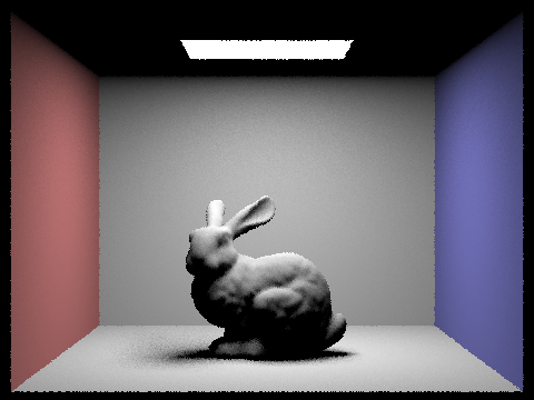
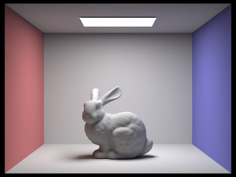
Task 4: Direct Lighting by Importance Sampling Light

Since hemisphere sampling was a little noisy, I implemented importance sampling with lights in order to get a more accurate representation. I calculated the same hit_p and w_out, but this time I attempted to compute the irradiance for each light in the scene. First, I checked if the current light was a delta_light, or a point light, in which case I only sampled once. Otherwise, I sampled for ns_area_light number of samples. For each one of the number of samples then, I first computed the radiance by plugging into the helper function sample_L(...) to get a the vector w_i, the distance to the light, and the pdf of the sample. Next, I checked if the the w_i in object space, which was the vector between the hit_p and the light source, had a z value less than zero, in which case the vector would be behind the object and we can ignore it. Otherwise, I formed a shadow ray from the hit_point and w_i, both in world space, set the max_t of the ray to disToLight - EPS_F, and set the min_t to EPS_F. From this I made sure that the shadow ray did not intersect my BVH. If it did, I ignored calculating the irradiance since I wanted to form a shadow, but if it did, I used the same reflectance equation as before to solve for L_out. For each light, I summed up all the samples I took, and then at the end, I summed up the values from each light to get the resulting illuminations. Below are some examples of this lighting:

Additionally, I tested and observed the results of the bunny using direct light importance sampling using 1, 4, 16, and 64 light rays respectively, with one sample per pixel. Notice how the noise in the image is significantly reduced as we use more and more rays, resulting with a better average:

Overall, the results with hemisphere sampling, while faster, usually resulted in a more noisy result. Sampling uniformly across the entire hemisphere can lead to interesting, but bad interactions with noise, whereas sampling with direct light importance only takes the light sources, which is valuable when dealing with more complex geometries. It is a tradeoff between speed and quality of image, although it seems like with the processing power of real uses of such lighting, its defintely more valuable to render the less noisy image at a slower pace.

Part 4: Global Illumination

Although direct illumination by itself is still pretty good, global illumination is even more realistic, representing light as it bounces throughout a scene. I implemented this by implementing indirect illumination, using a recursive style function, literally tracing the path the ray takes when it bounces between surfaces. First, I defined w_out and hit_p in the same manner as previous functions, and also initialized L_out to be the spectrum of using direct illumination using the current ray. This time however, I used the function sample_f(...) to get back a w_in ray in object space, as well as the pdf of sampling that ray. Converting this into world space, I use that as the direction to define a new ray with origin hit_p, with a depth one less than the depth of the input ray. Next, I checked the conditions of pdf > 0 (to prevent dividing by zero) and that the new ray intersects the BVH. Following this begins the recursive process. If the depth of the inputted ray to the function equaled the maximum ray depth, this was the very first call, and I made it calculate the effect of bouncing at least once. For this, I used the same reflectance equation as before, taking the recursive value times the BSDF emission times the cosine of w_in in object space, divided by the pdf. If the ray's depth was less than the maximum, then this was not the first bounce; for this, I implemented a Russian Roulette style termination scheme, where with a probability of 0.6 I continued to recursively bounce the ray and update the radiance value. Sampling from that distribution, if the depth was still greater than 1, then I used the same reflectance recursion to update L_out, only this time dividing by the continuation probability as well to normalize. I could then eventually return L_out as intended. The recursion is never infinite because the maximum number of times that we can follow the path is set as the max_ray_depth, and additionally the Russian Roulette will also stop paths prematurely as well.

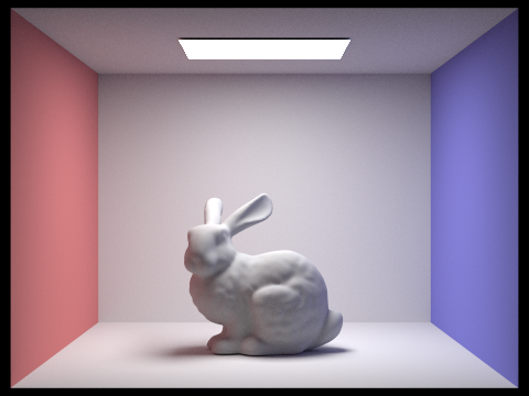
Below are examples of global illumination, using a combination of direct and indirect illumination, with 1024 samples per pixel:

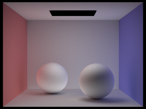
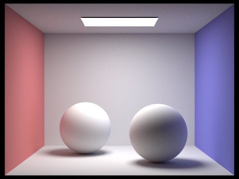
Additionally, below are the Lambertian Spheres, the first rendered using only direct illumination, the second using only indirect illumination. Notice how the direct lighting image has direct shadows cast due to the rays cast from the light source, while for the indirect lighting we see a soft light throughout the whole image. This is because the indirect illumination is literally just the effects of the bounces of rays, with no direct lighting from the light source's original rays.

We can see the effects of ray depth from the following renderings of the bunny, where we alter the maximum ray depth for each subsequent render. Notice that each one lets more and more light into the scene, but eventually there is very minimal tradeoff since the probability of a ray actually getting to bounce a large number of times is very small by the Russian Roulette:

Lastly, I also rendered the spheres once again using varying sample-per-pixel rates. Notice that increasing the sample size will significantly decrease the noise that is involved within the rendering:

Part 5: Adaptive Sampling

Since some pixels will naturally converge faster than others, we can reduce overall noise by sampling pixels that converge earlier less than those that need to converge later. The technique for this is adaptive sampling, where for each pixel, we individually determine if its average illuminance is between [mean - I, mean + I] with 95% confidence, where I = 1.96 * (standard_deviation / sqrt(n)). Essentially, for this process, I compute a running sum of illuminances of samples s1, as well as a running sum of illuminances squared s2. Then, for every samplesPerBatch number of samples, I calculate the mean of the number of samples, n, so far, s1/n, and the variance (1/n-1 * (s2 - (s1 * s1 / n))). I use these to calculate the value I based on the previous equation before, since standard deviation is the square root of variance, and then check if I <= maxTolerance * mean, where maxTolerance is some specified constant like 0.05. If the condition holds true, we claim that the pixel has converged, and stop iteration at the current number of samples. We can then update the Spectrum average that we've accumulated so far by dividing by the actual number of samples that we took, and then updating the pixel in the framebuffer. Lastly, I update the sampleCountBuffer with the actual number of samples taken to get a sample rate image.

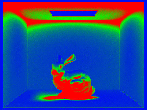
To demonstrate this, I rendered the bunny once again with 2048 samples per pixel, this time using adaptive sampling. Notice how the walls at the sides and the floor converge much faster than the bottom of the bunny and the ceiling surrounding the light source.