Part 1: Masses and Springs

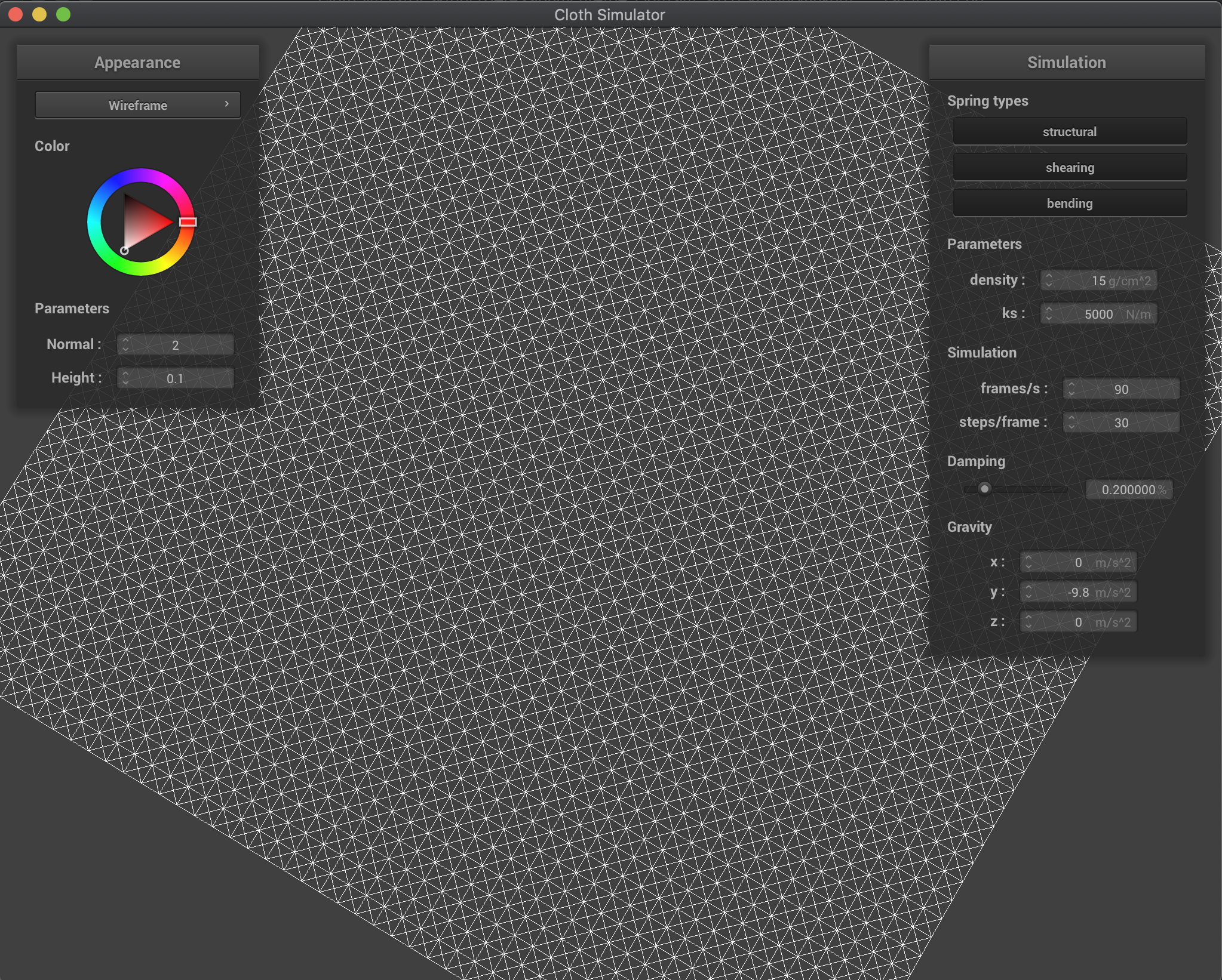
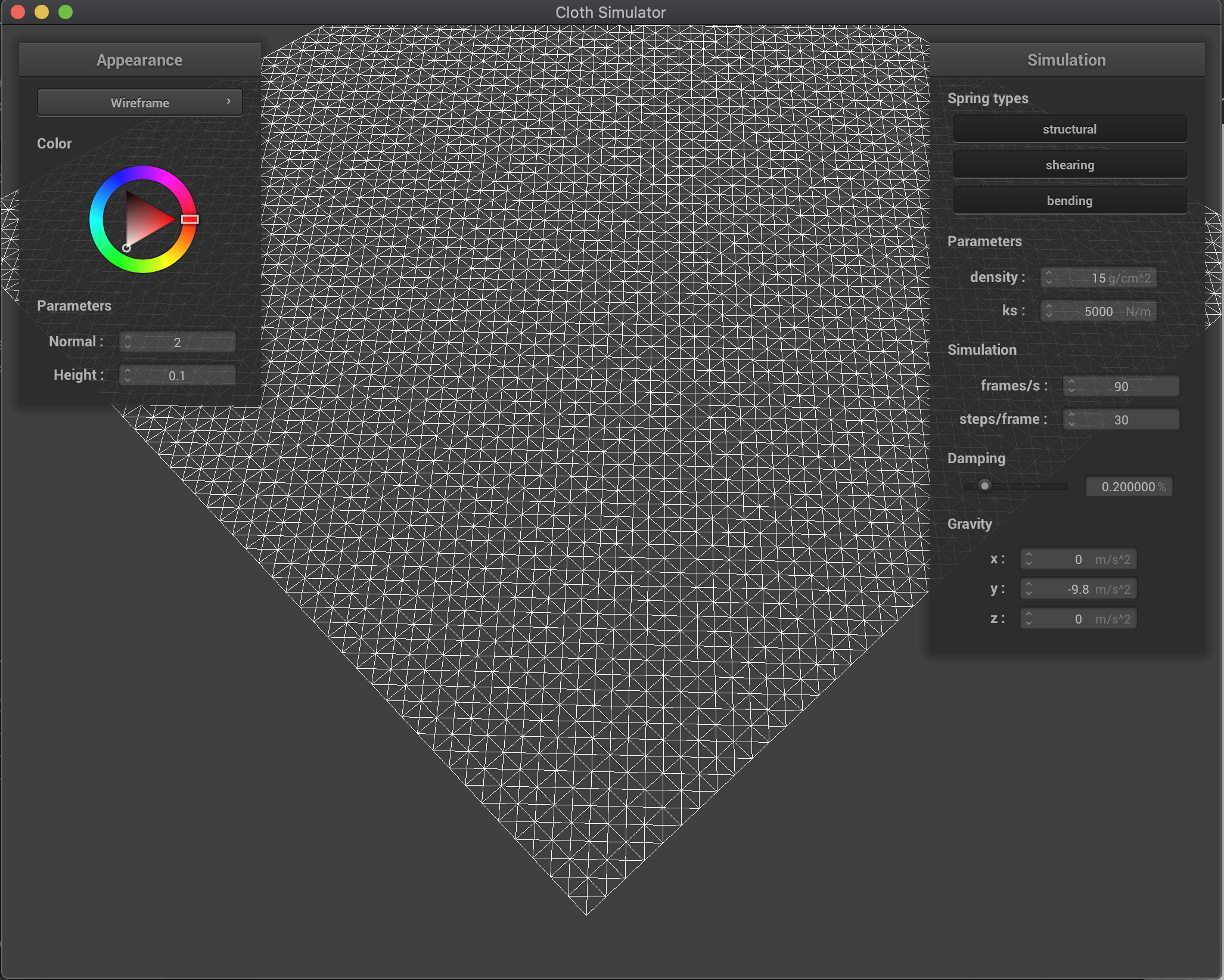
In order to begin simulation of cloth, I first needed to use a system of point masses and springs in order to create a model of a sheet of cloth with some chosen dimensions and parameters. In this part, given a width, height, and number of points in both dimensions of the cloth, I built a grid of equidistant point masses on a 2D plane, where each point mass was a point, and they were connected by springs. In the case that the cloth was horizontal, I set the y-axis to always be the same (1), and that varied points along the x and z axes. For a vertical cloth, I used a small offset on the z-axis, and then varied points along the x and y axes. After constructing establishing all the point masses, and setting chosen point masses to be pinned, I connected them with springs that represented different constraints depending on how the two point masses were connected. Point masses to the left and above of each other used structural constraints, point masses diagonal upper left and upper right from from each other used shearing constraints, and point masses two points to the left of each other used bending constraints.

Below are the results of creating this model. First is the result of building the grid for the given scene/pinned2.json, from different viewing angles:

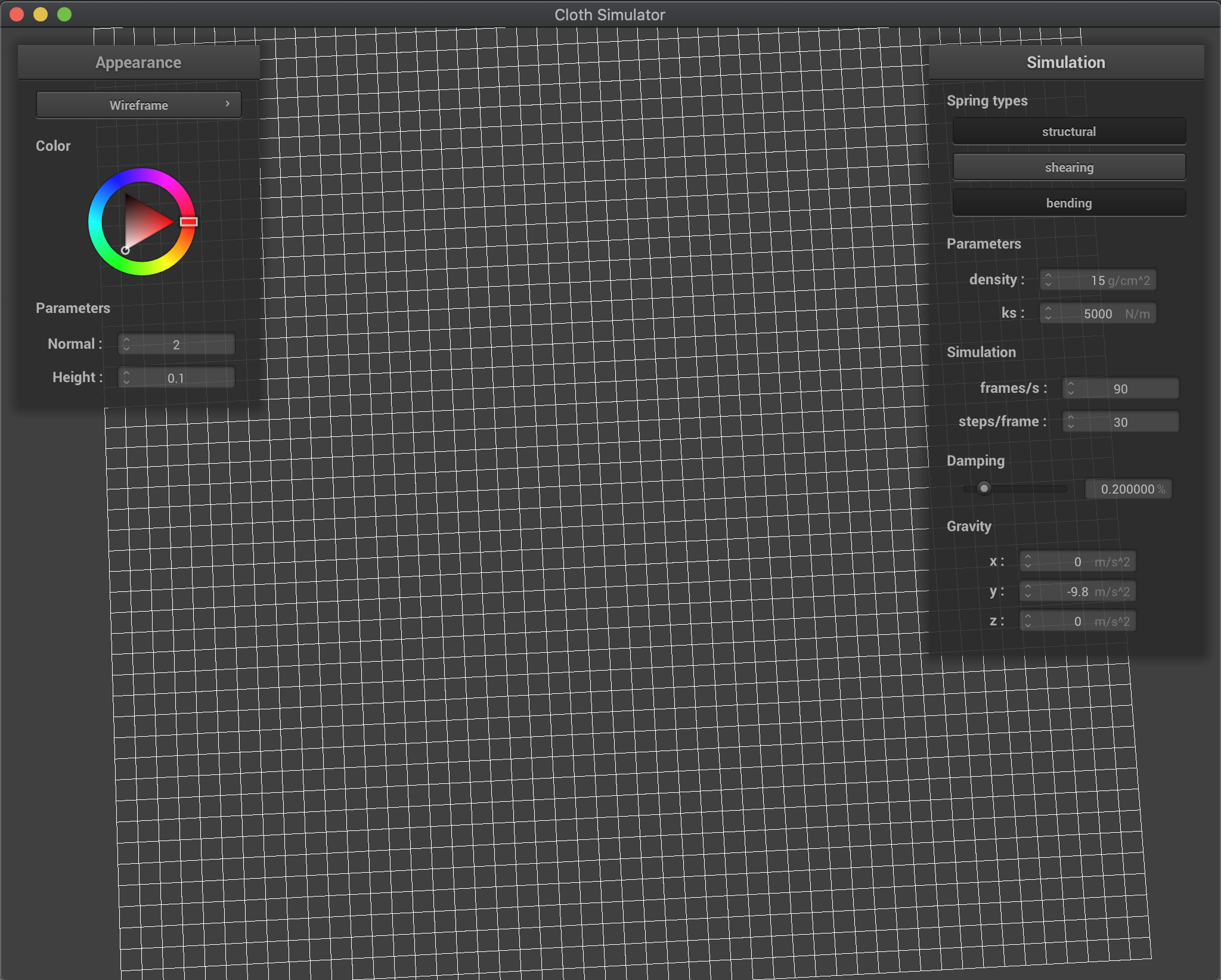
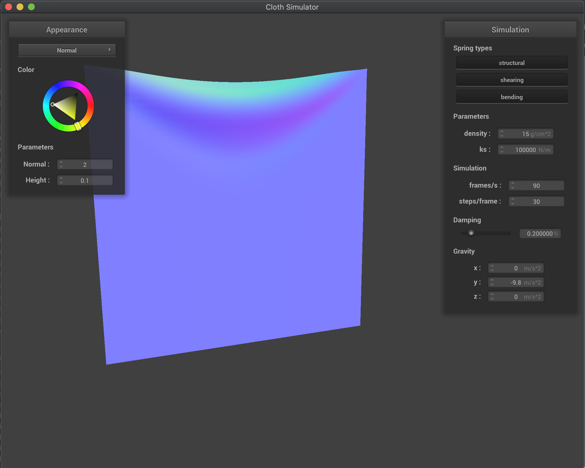
Now below is the result of building the model for scene/pinned4.json, with various constraints active at a given time:

Part 2: Simulation via Numerical Integration

For this part, I was able to mimic both external forces and spring correction forces acting on a cloth to demonstrate the motion of a cloth held up by pins as it goes to rest. First, I computed the total external force based on the given external_accelerations and mass and applied that force to every point mass in the grid. Then I iterated through the springs, and computed the relevant force using Hooke's Law, then applying it in opposite directions to each point mass connected by the spring.

After doing this, I then used Verlet integration to get new point mass positions after applying the calculated total force to each point mass. Through this, I calculated the next position based on the position from the previous time step, a damping factor, the acceleration, and the time step delta_t. Lastly, I made sure to constrain the positions after this update, so that the distance between each pair of point masses did not exceed 1.1 times the resting length of the spring. To calculate this, I computed the normalized direction vector between the two points, and scaled the positions accordingly using this vector.

I then observed the effects of altering parameters on the simulation. Below are the results of using both a very high spring constant, k_s, and a very low one. The spring constant relates directly to the stiffness of the springs, and as such, a high one makes the cloth stiffer, and a low one makes the cloth more elastic and stretchy. This is noticable both in the simulation, and at rest, where the higher spring constant results in a much more rigid cloth than the lower one:

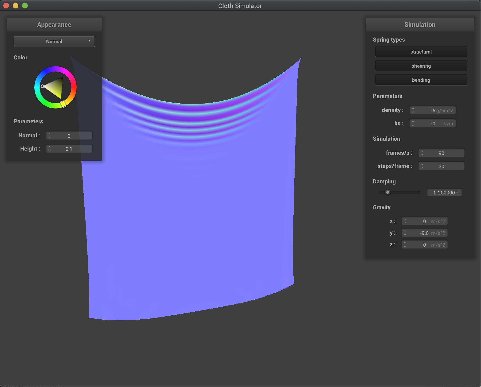
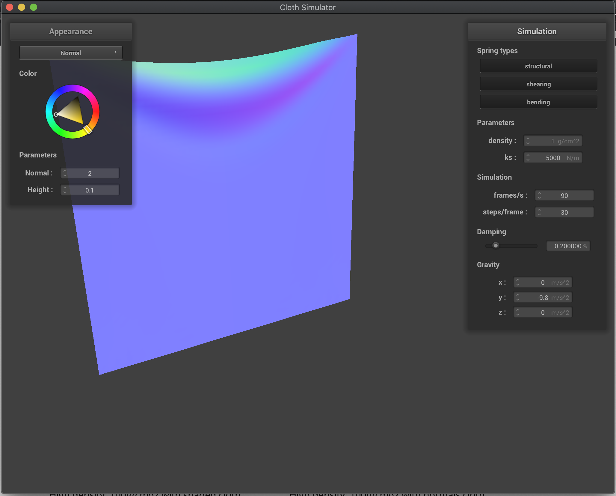
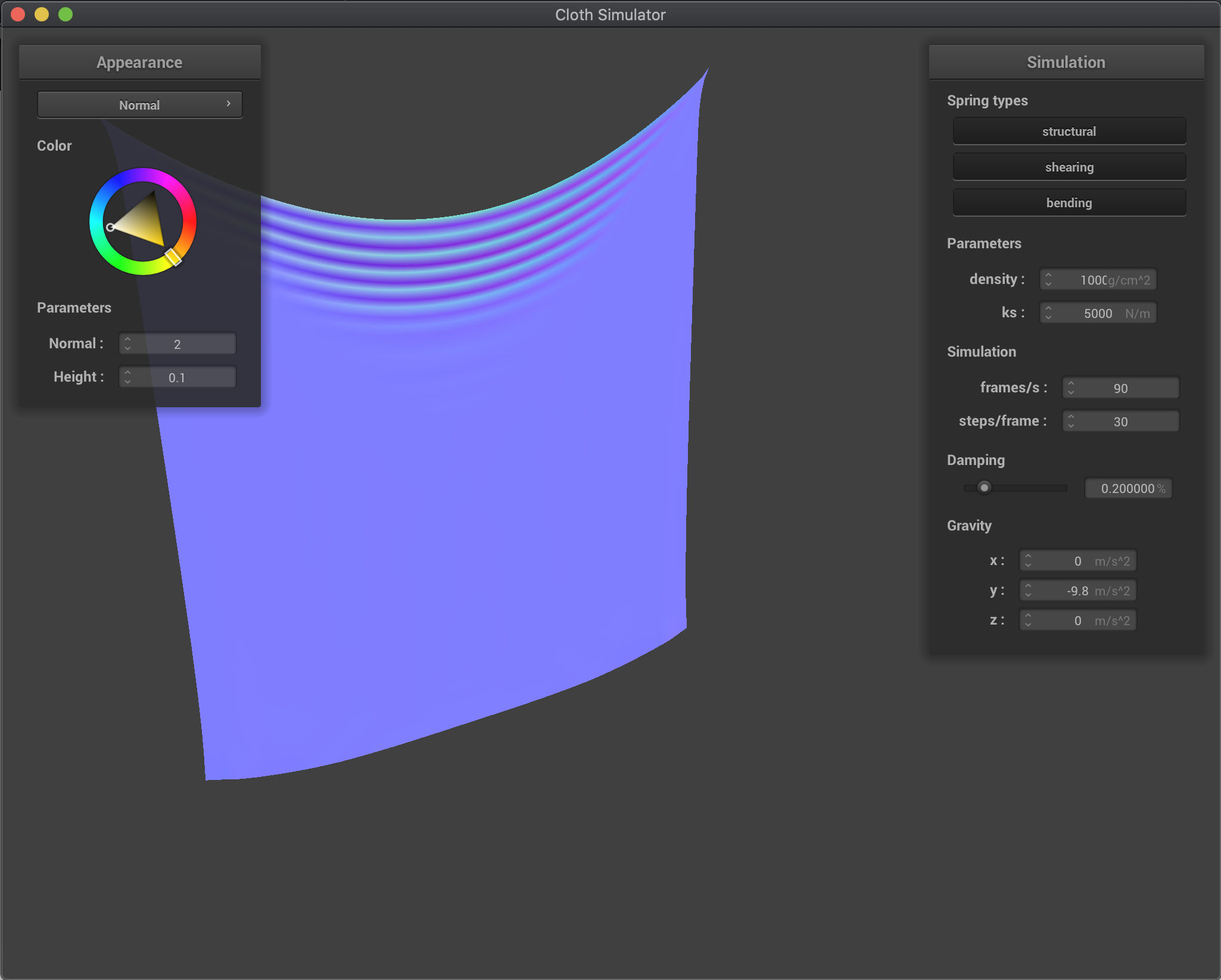
Next, I tested the effects of varying density. A low density as seen in the first image results in a lower mass, and as such less force acting on the cloth. This can be seen as the cloth itself looks a lot lighter with slighter curves. In constrast, the high density cloth has a lot more force acting on it, resulting in a stiff, heavy result. Additionally, the deeper curves are a result of the heavier mass at each point:

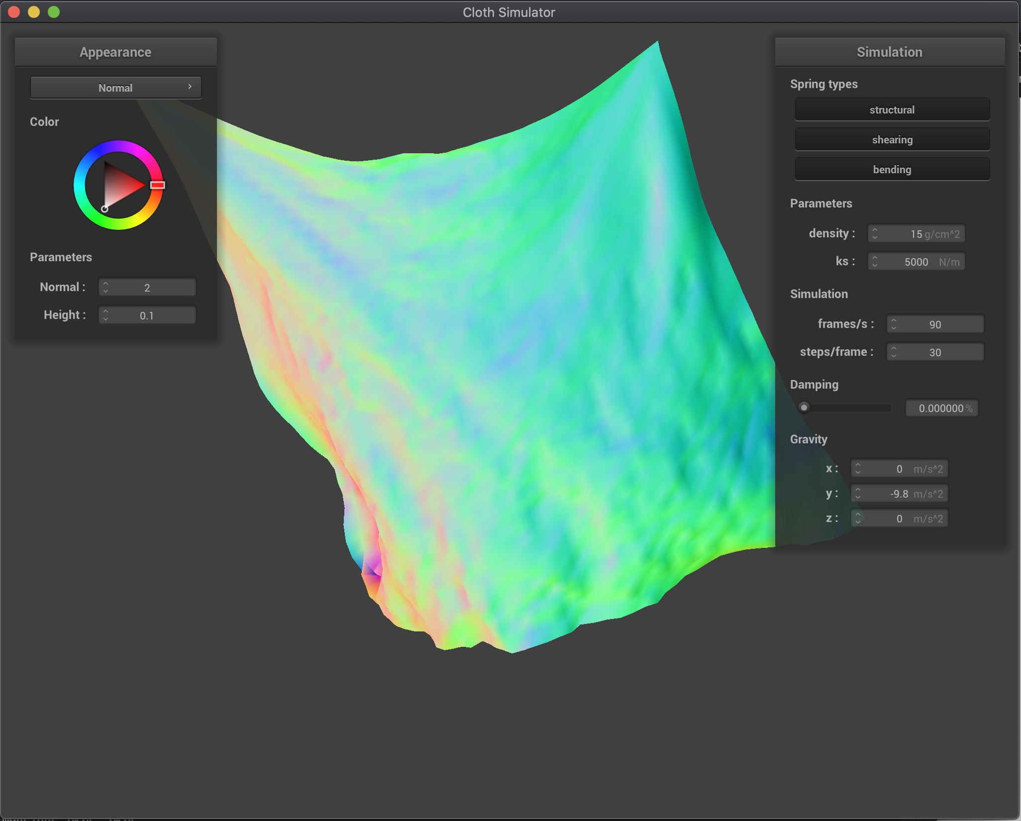
Lastly, I experimented with the damping constant, from 0 to 1. Since the damping constant relates to how quickly energy is lost in the cloth, a higher damping constant results in a quicker convergence to steady state, whereas a lower damping constant results in a longer time to converge. Additionally, the lower damping constant close to 0 means that the cloth will sway almost indefinitely, while a higher damping constant like 1 means that energy is immediately lost and the cloth will almost immediately stop swaying:

Last but not least, here is the result of simulating a cloth with 4 pins with regular parameters:

Part 3: Handling Collisions with Other Objects

Now for my simulations, I modeled the effects of the cloth colliding with objects, specifically both spheres and planes. To handle collision with a sphere, I computed the correction vector by first computing the direction vector. If the direction vector has a norm less than the radius of the sphere, this means that the original point is inside the sphere, so I build the correction vector with respect to the direction, radius, origin of the sphere, and the point's current position. I then update the position by multiplying the correction vector by 1 - friction, which helps to scale down the new position, and then add that to the last position of the point mass.

For colliding with a plane, I first found the distance between the point and the plane using a dot product with difference in position between the point mass and the plane's defining point, and the norm. If this value was negative, this means there is a collision, so I subtracted the SURFACE_OFFSET from this distance, and then computed the correction vector by multiplying this by the normal of the plane, then subtracting this from the point mass's position, and then subtracting the point mass's last position. Finally, I used the correction vector to update the position, with the same process as the sphere, where I multiplied the correction vector by 1 - friction and then added that to the last position of the point mass.

Below is the result of tweaking the spring constant k_s before running the simulation for collision with the sphere. The first image depicts a low spring constant, and we can see that the lack of resistance within each spring allows the cloth to drape more and adapt closer to the actual smooth surface of the sphere. The second image depicts a regular spring constant, and here we see the most normal looking cloth being held up by the sphere, draping at a very natural position. The spring constant allows for the cloth to sit regularly, as it is neither too stiff or too loose. The third image shows the result of a high spring constant, which causes more stiffness in the cloth. Here, the cloth wants to keep its own geometry rather than conforming to that of the sphere, which shows in how the cloth lays at rest in a more rigid fashion:

Additionally, this is the result of simulating the cloth's collision with a plane. Note that the further below two images were taken after being able to customize the cloth using shaders properly in Part 5:

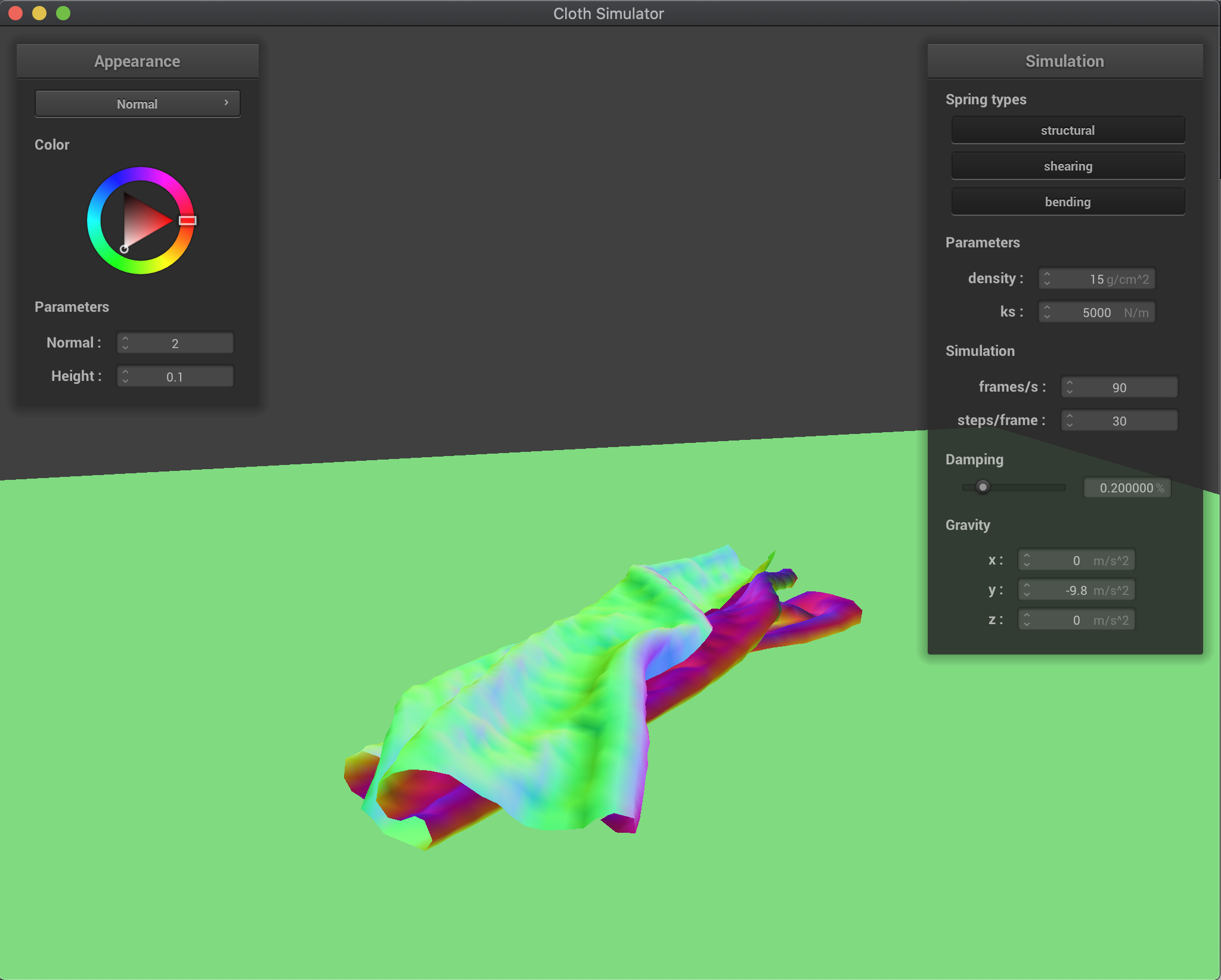
Part 4: Handling Self-Collisions

Originally, the simulation did not take into account self-collisions of the cloth, resulting in the cloth folding into itself. In order to fix this, I implemented spatial hashing and computed between point masses whether they were a certain distance apart, 2 * thickness. If they were not, I applied a correction force to the point mass in question in order to make sure they were. To do this, I created a hash function to map points to box regions within the 3D space, and then stuck them into a hashmap. Then for each point mass, I found its corresponding box, and computed the average force I needed to apply to it based on all the other point masses in the box. After doing this, the cloth no longer folds into itself!

First, here are the general results of the simulation after implementing proper self-collision. Notice how the cloth doesn't fold into itself, and kind of naturally folds around until it reaches a relative resting point:

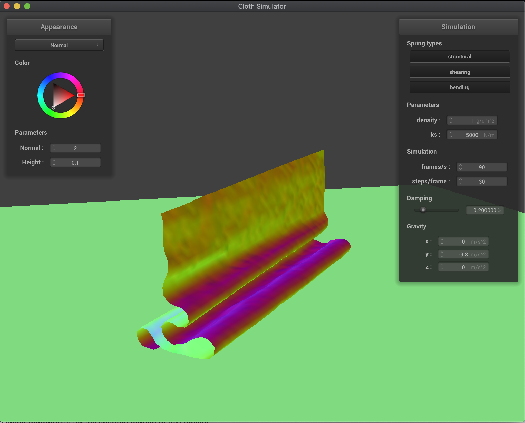
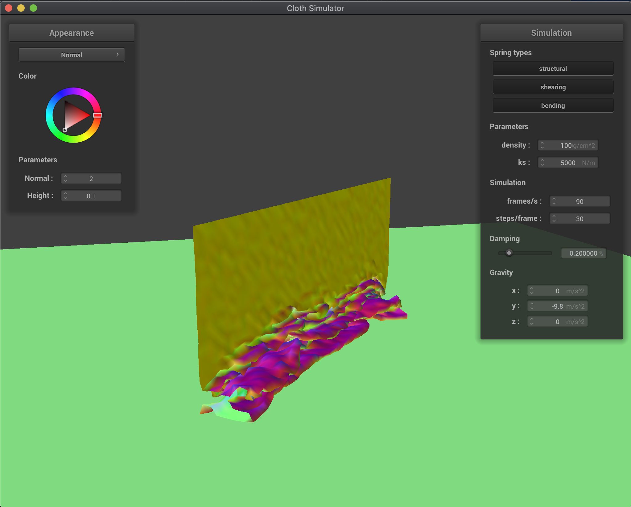
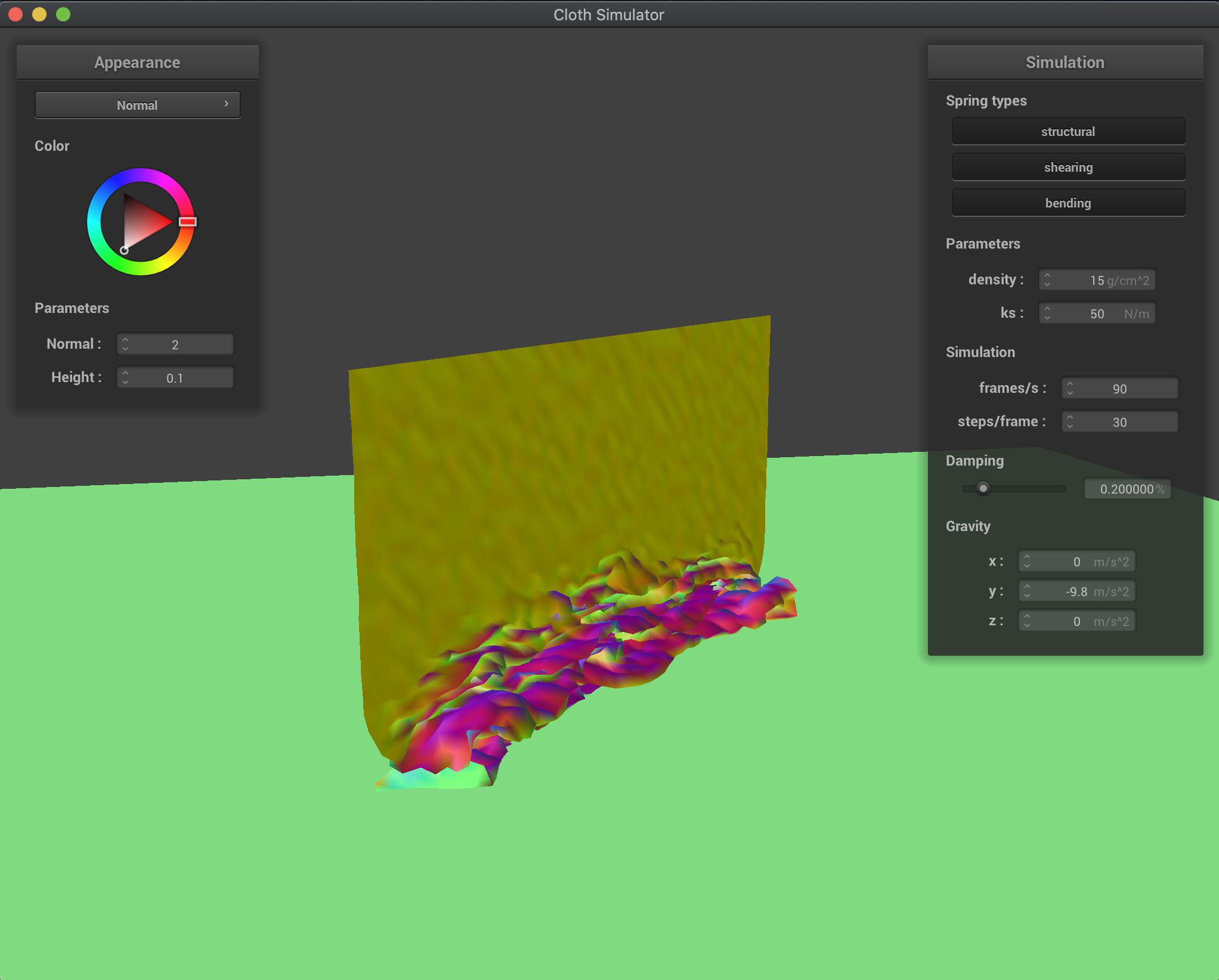
Next, I experimented with the results while tweaking both the density of the cloth and the spring constant. As before, lower density results in a lower mass, which means less force acts on the cloth, and allows it to go down lightly with bigger folds; on the other hand, higher density results in a higher mass, or more force, and makes the cloth fold faster and with smaller folds:

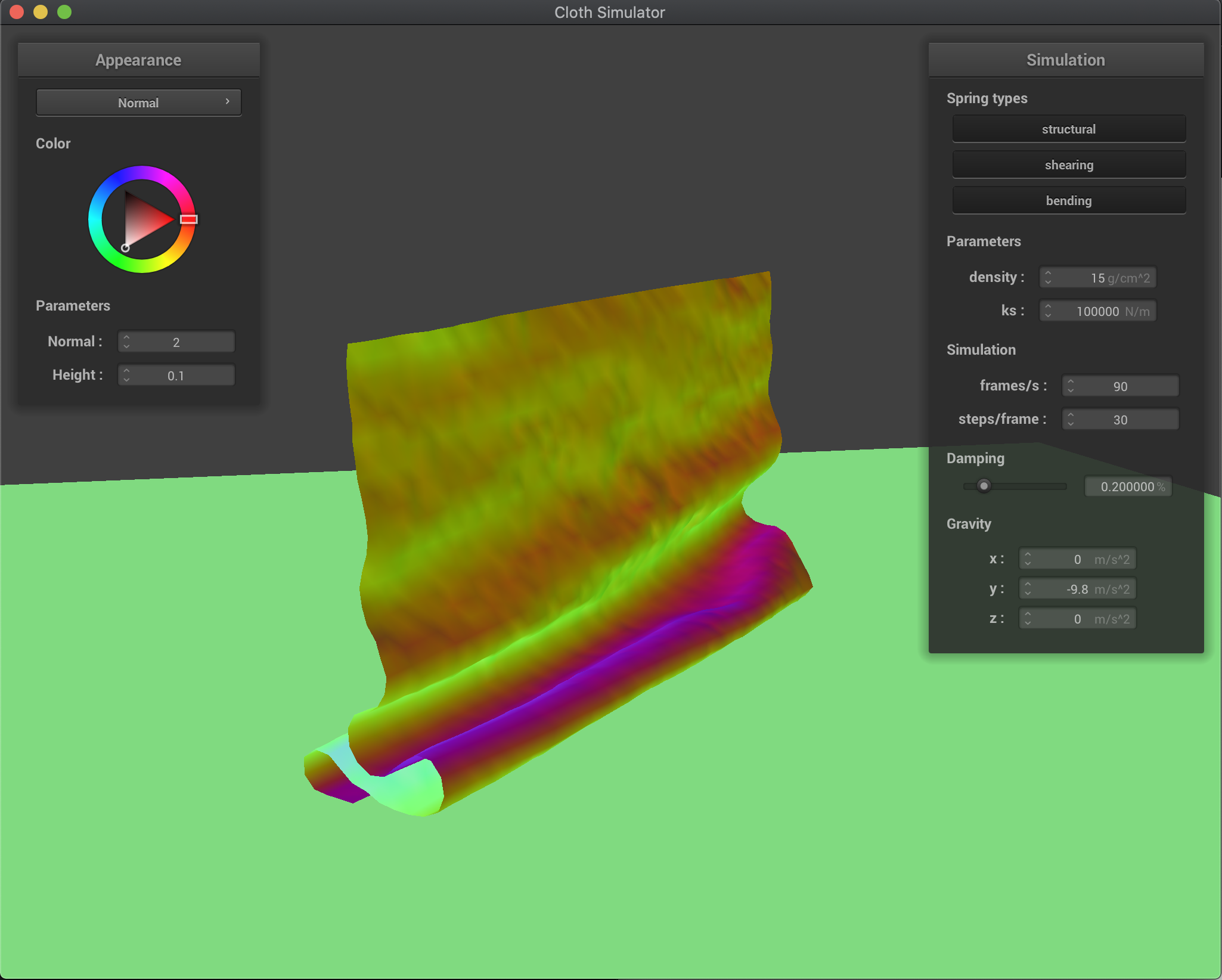
In a similar relationship, a lower spring constant meant that the cloth was more springy, folded less, and took longer to reach its resting state, whereas a higher spring constant meant that the cloth was stiffer, folded more, and reached its resting state much more abruptly:

Part 5: Shaders

After fully implementing collision detection, I implemented shaders in order to make the surfaces of the cloth more distinct and unique. Basically, a shader program is a program that is run in parallel on a GPU that takes in inputs, and outputs a single four dimensional vector. This can be done much faster than raytracing on the CPU, and allows us to do that similar thing at a much faster and more efficient rate.

To create a shader program, we need to create and combine both a vertex and a fragment shader, where whatever is the output value of the vertex shader will eventually become the new input value of the fragment shader. A vertex shader applies geometric transforms to vertices and points, altering things like position of vertices, normal vectors, and various other things. It will then output the final position of the vertex its operating on as the value of gl_Position, which will then later be used for the fragment shader. A fragment shader will take geometric properties of a specific fragment that its operating on, which is created after rasterization, and then from there computes the appropriate color of the fragment. It then outputs that color value, which will then be used to color in the material.

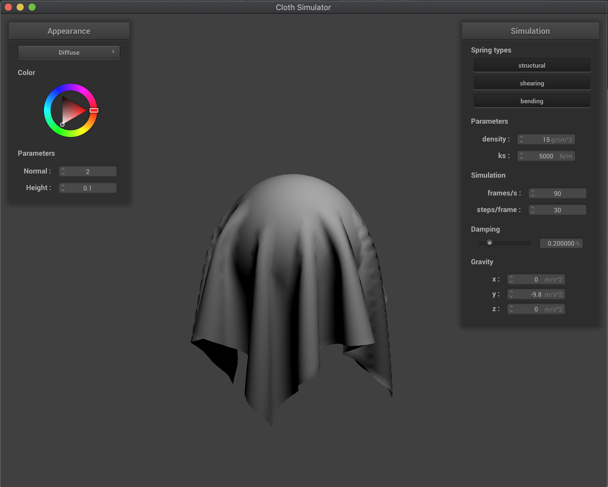
Task 1: Diffuse Shading

The first shader program I wrote was for diffuse shading, in which I used the equation from lecture L_d = k_d * (I / r^2) * max(0, dot(n, l)) in order to get the appropriate shading. Taking in the inputs writing the result of that equation into my color vector gave the following style of image:

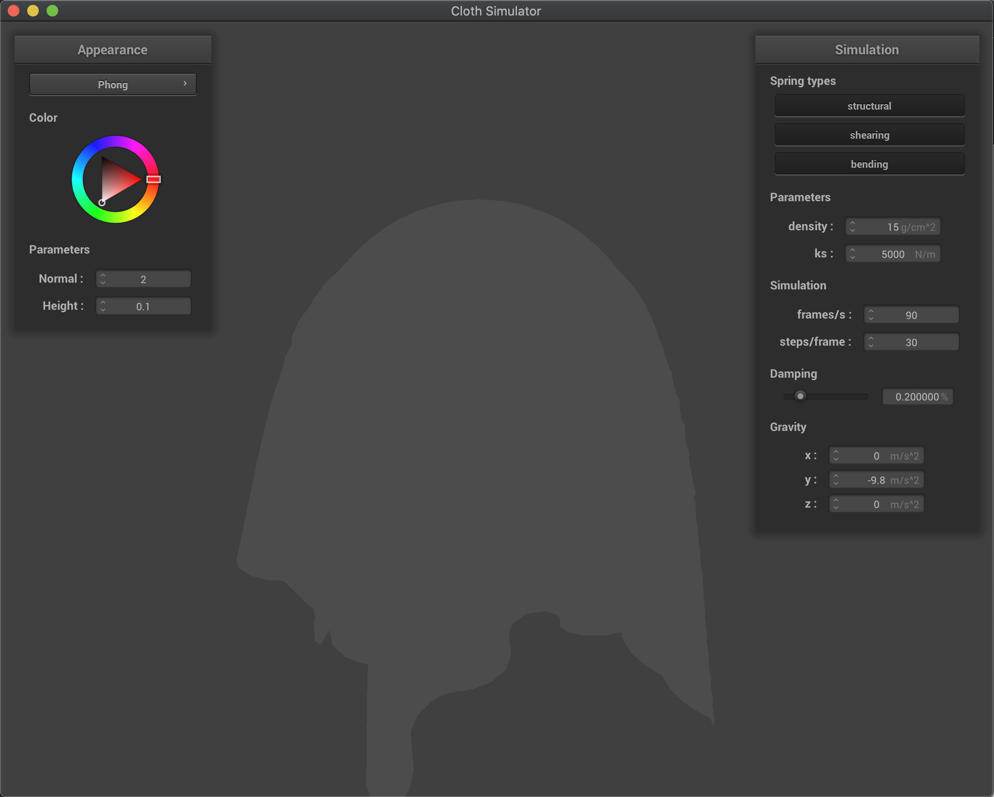
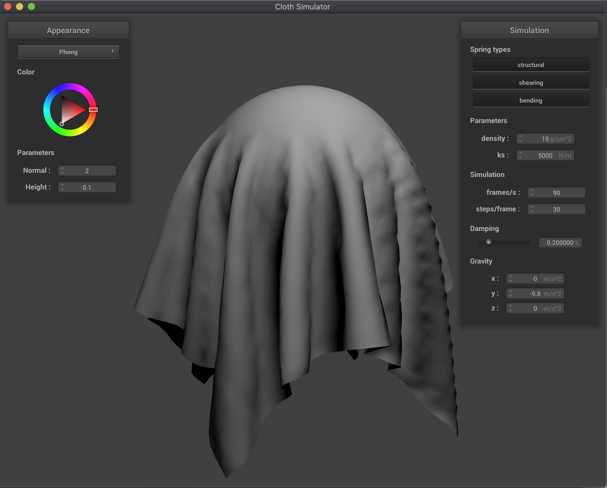
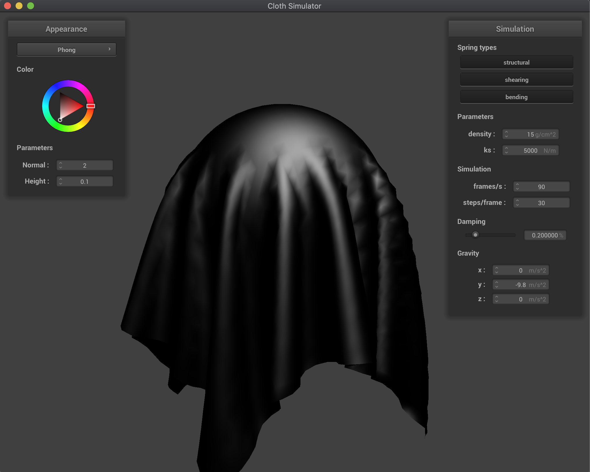
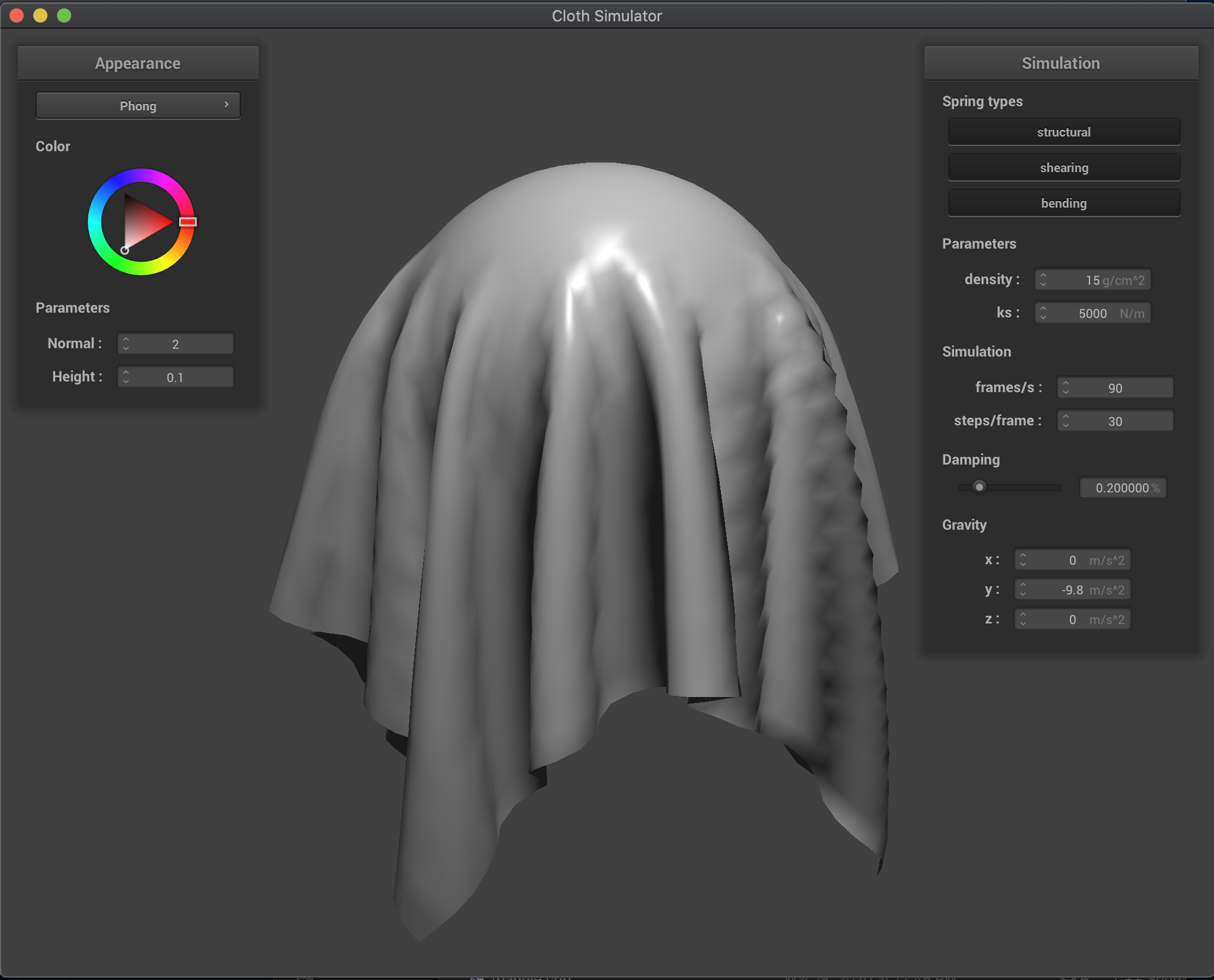
Task 2: Blinn-Phong Shading

The next shader that I wrote was for the Blinn-Phong shading model as described in lecture, essentially in this model, we account for ambient lighting, diffuse lighting (same as in the previous shader), and specular highlights, in order to get a properly shaded model, that looks like it has lighting effects. Each of these can be solved for separately, and as such, we can show what the impact of each piece has visually. I used the equation L = k_a * I_a + k_d * (I / r^2) * max(0, dot(n, l)) + k_s * (I / r^2) * max(0, dot(n, h))^p to find the result, where each subpart in between additions is ambient, diffuse, and specular respectively. For my parameters, I chose k_a = 0.3, I_a = 1.0, k_d = 1.0, k_s = 0.5, and p = 100.0. The results of each part individually and all combined are below:

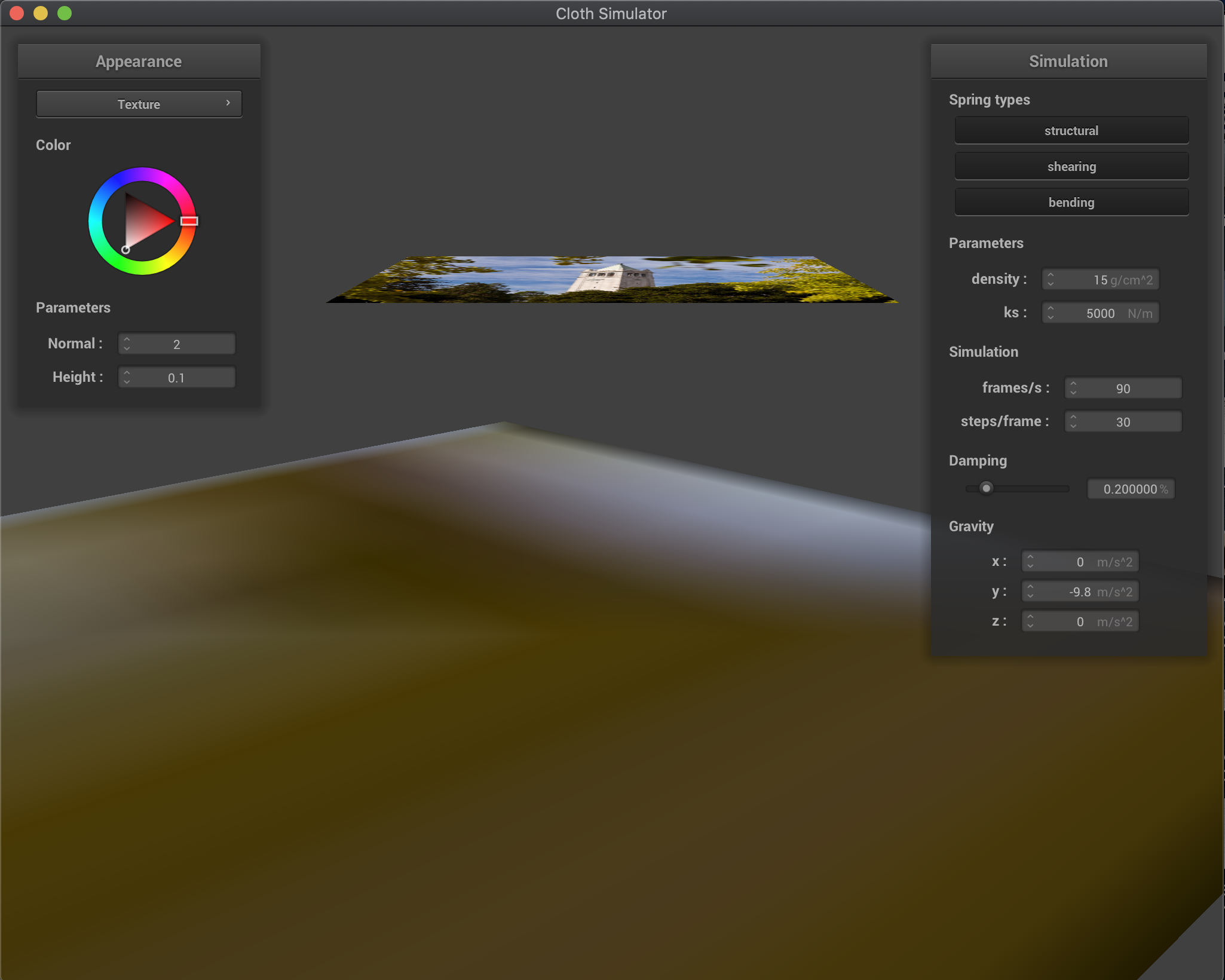
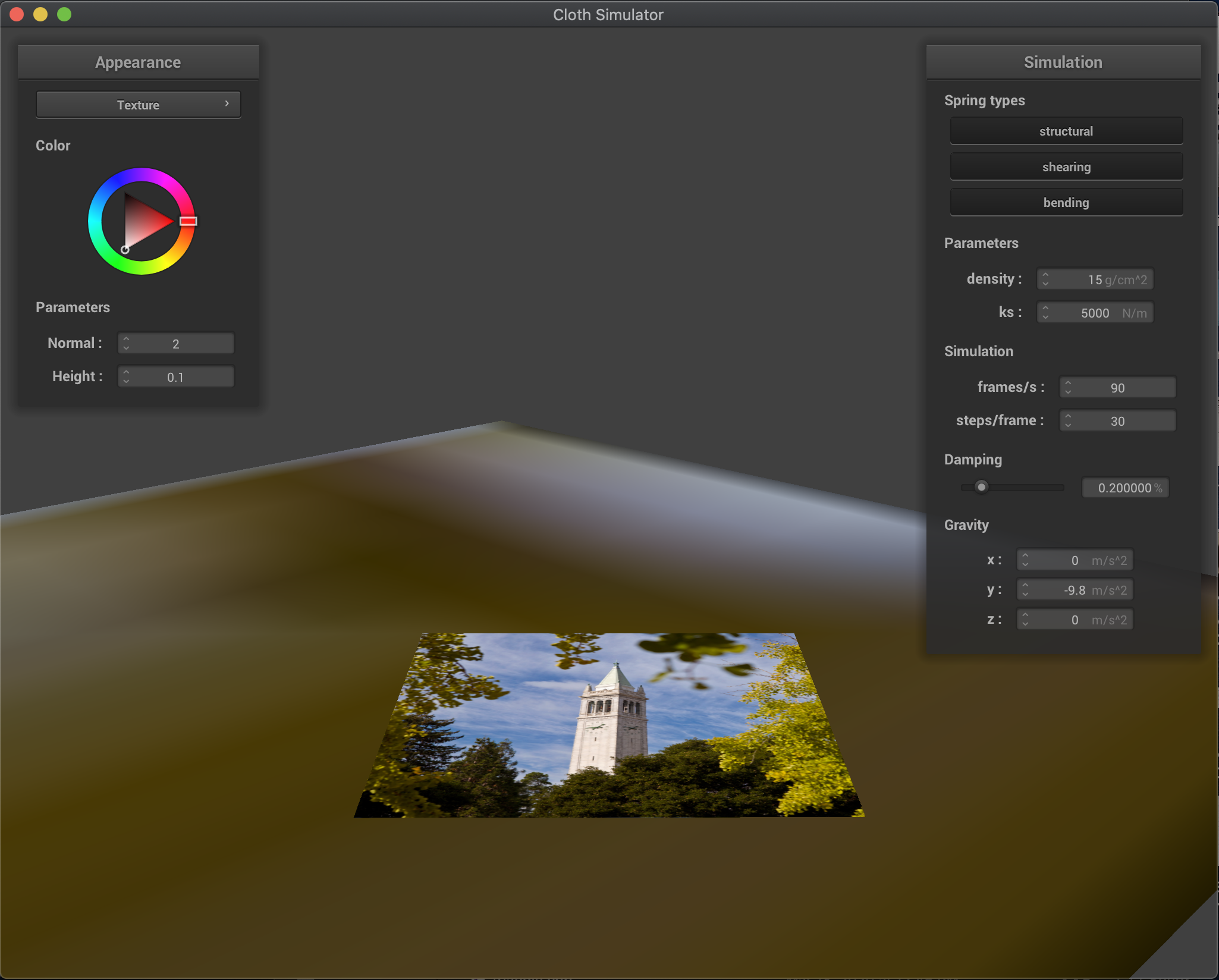
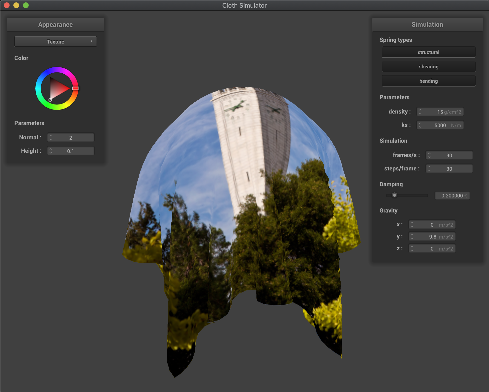
Task 3: Texture Mapping

For my next shader, I sampled uniformly from a given texture at a given uv coordinate and outputted that color, in order to appropriately map a texture to the surfaces. Below are the results of the default texture mapping, as well as a customized one:

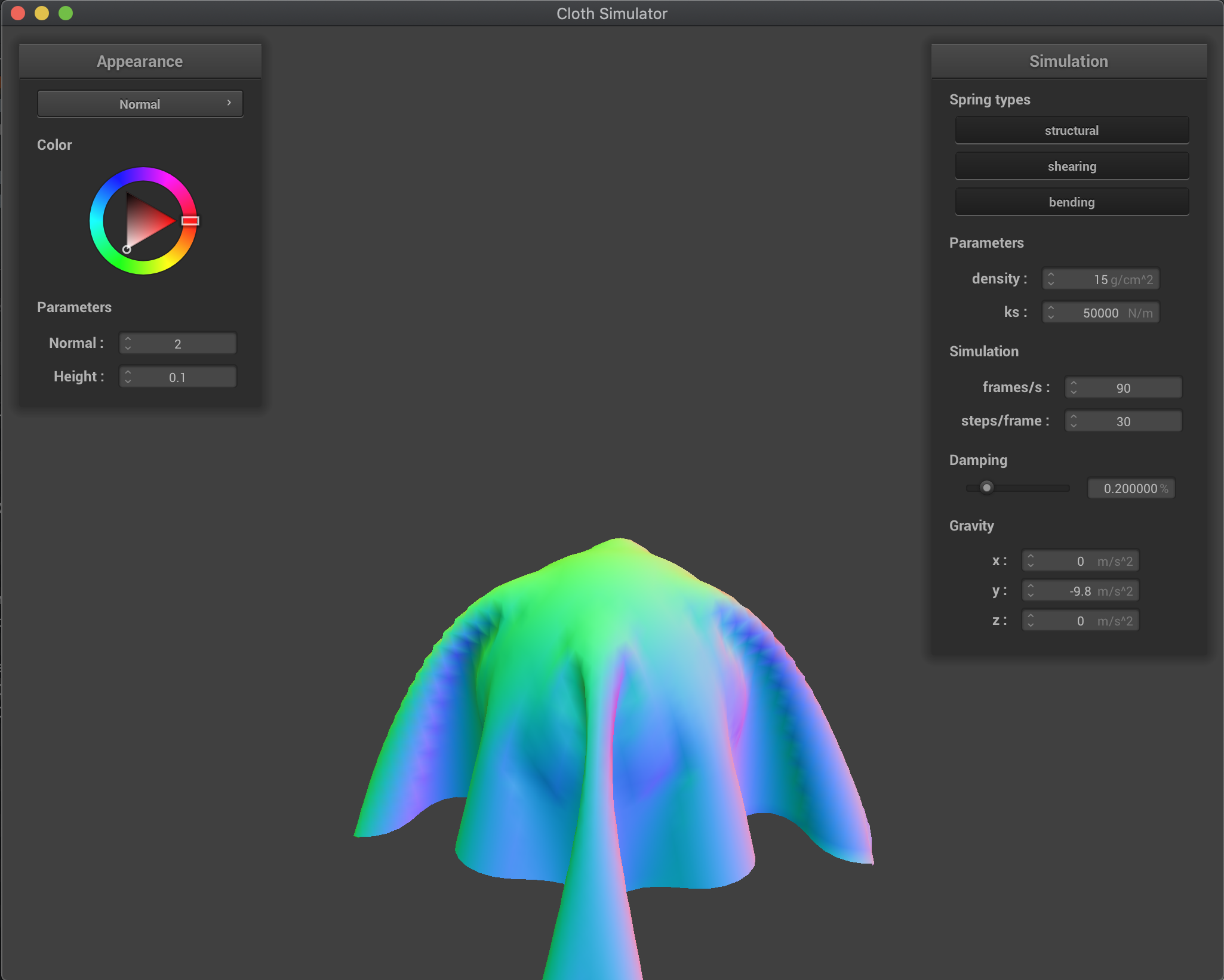
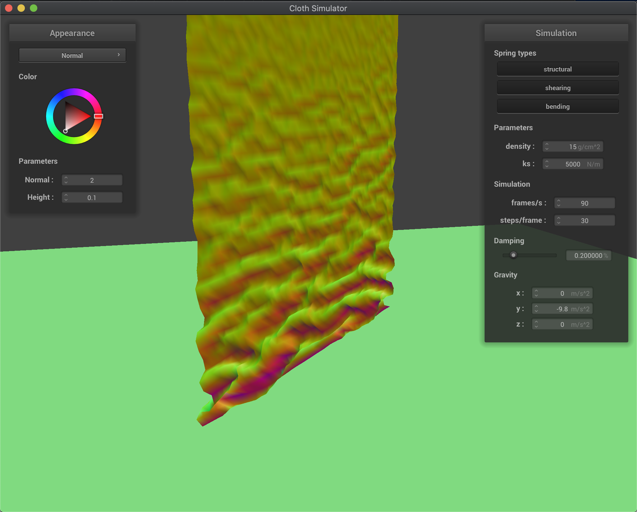
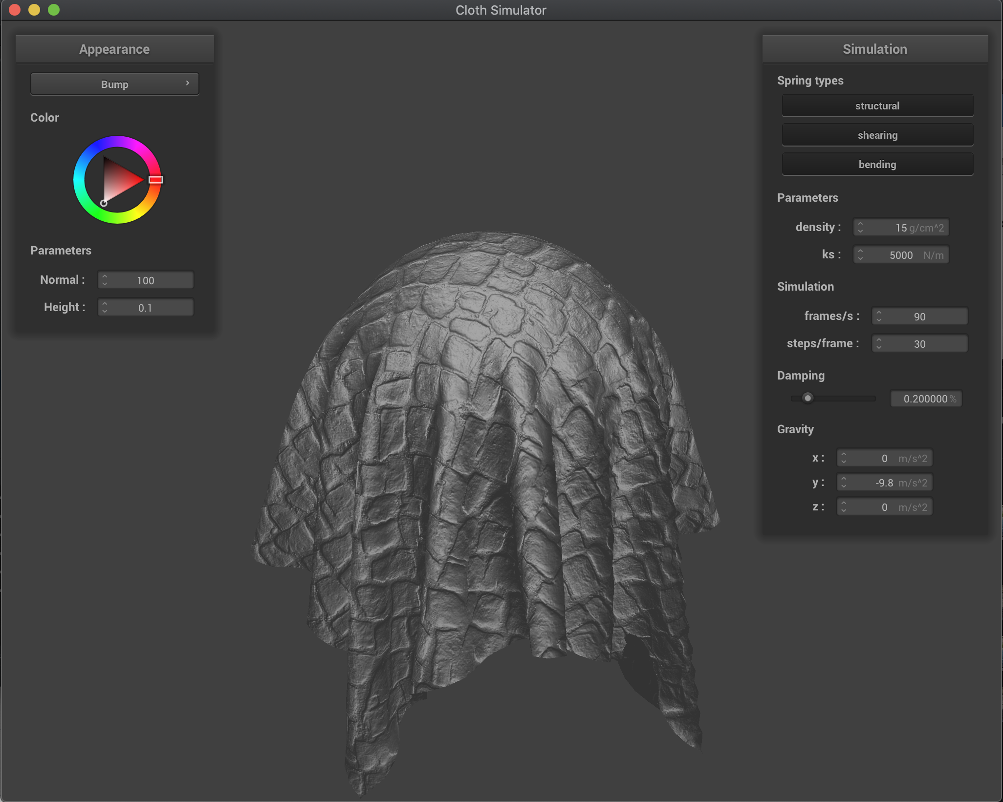
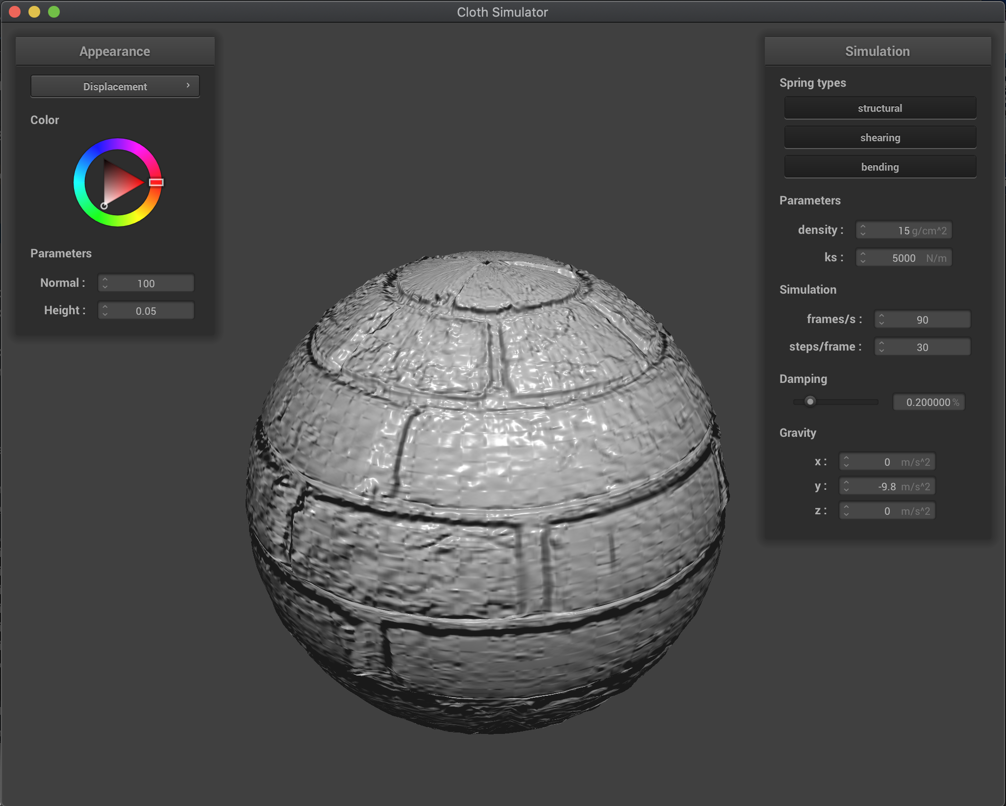
Task 4: Bump and Displacement Mapping

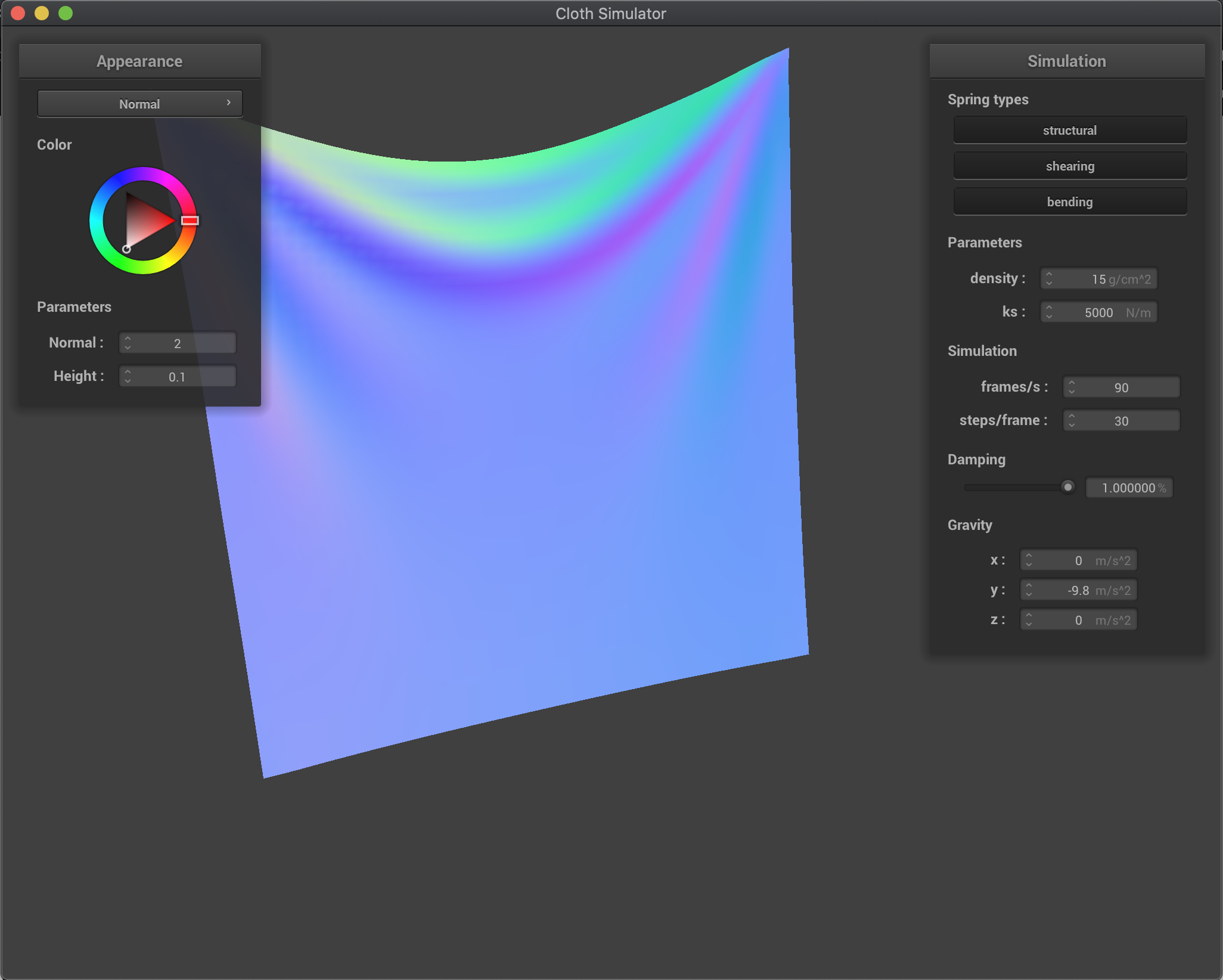
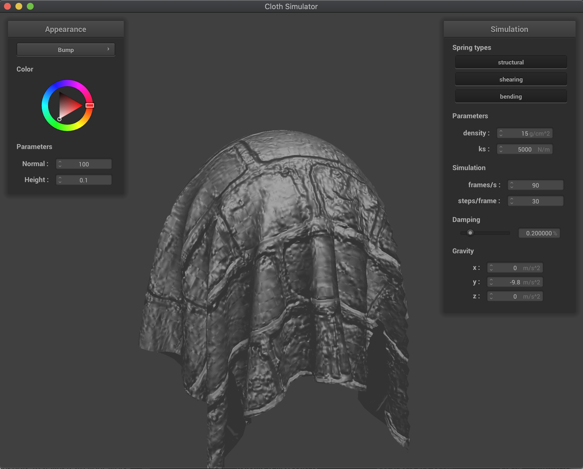
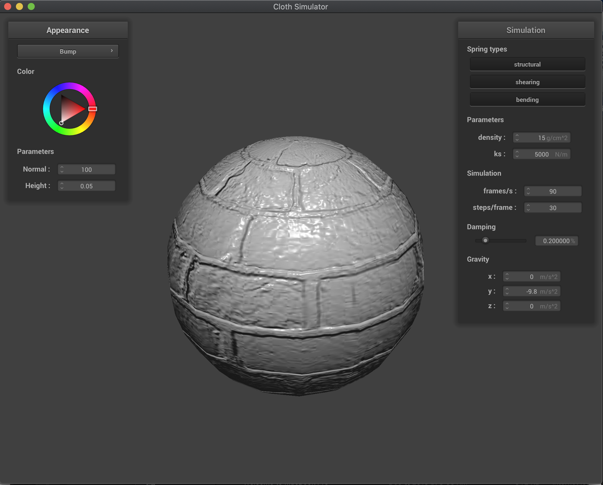
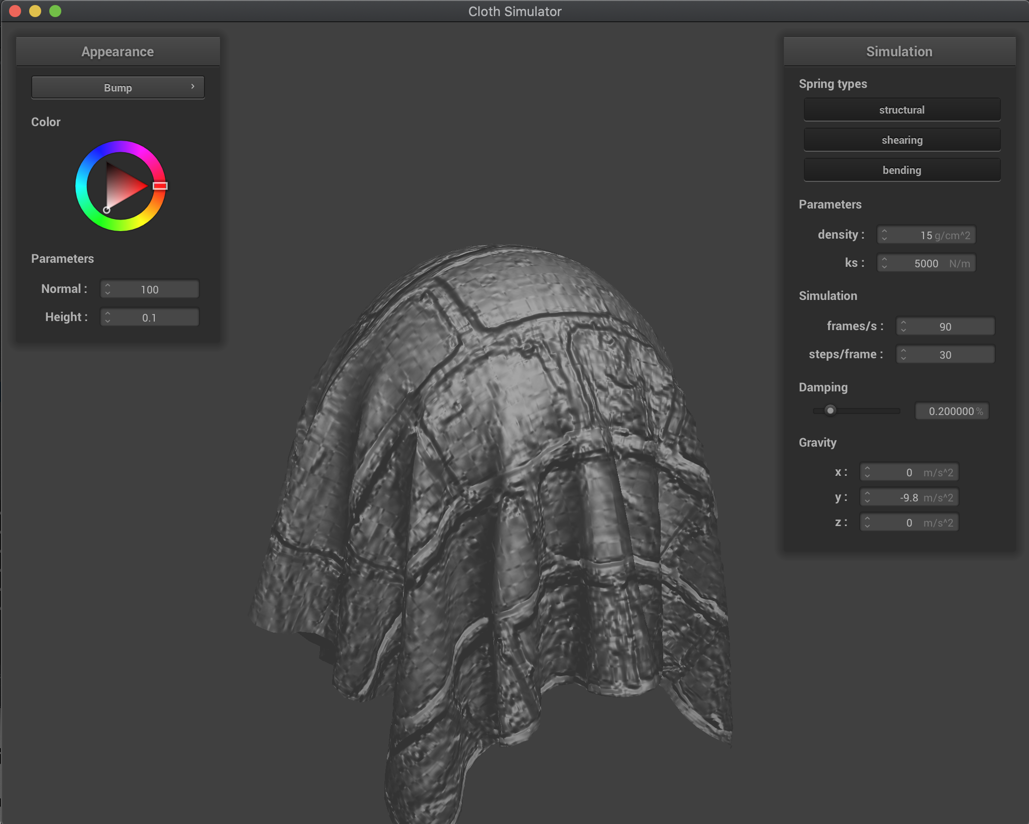
For my next two shaders, I took a processed height map in order to compute a normal mapping, and then applied this mapping to my model. For bump mapping, I computed a displaced model space normal using a tangent-bitangent-normal (TBN) matrix and applying that matrix to the local space normal n_o = (-dU, -dV, 1), where dU = (h(u + 1/w, v) - h(u, v)) * k_h * k_n and dV = (h(u, v + 1/h) - h(u, v)) * k_h * k_n. The function h(u,v) returns a height encoded by the provided height map at the texture coordinates u and v, and doing this allows us to find the corresponding normal to create realistic lighting effects. With that normal, I just used that normal in place of the regular one in the Blinn-Phong Shading Model in order to get a fairly realistic bumped map like below:

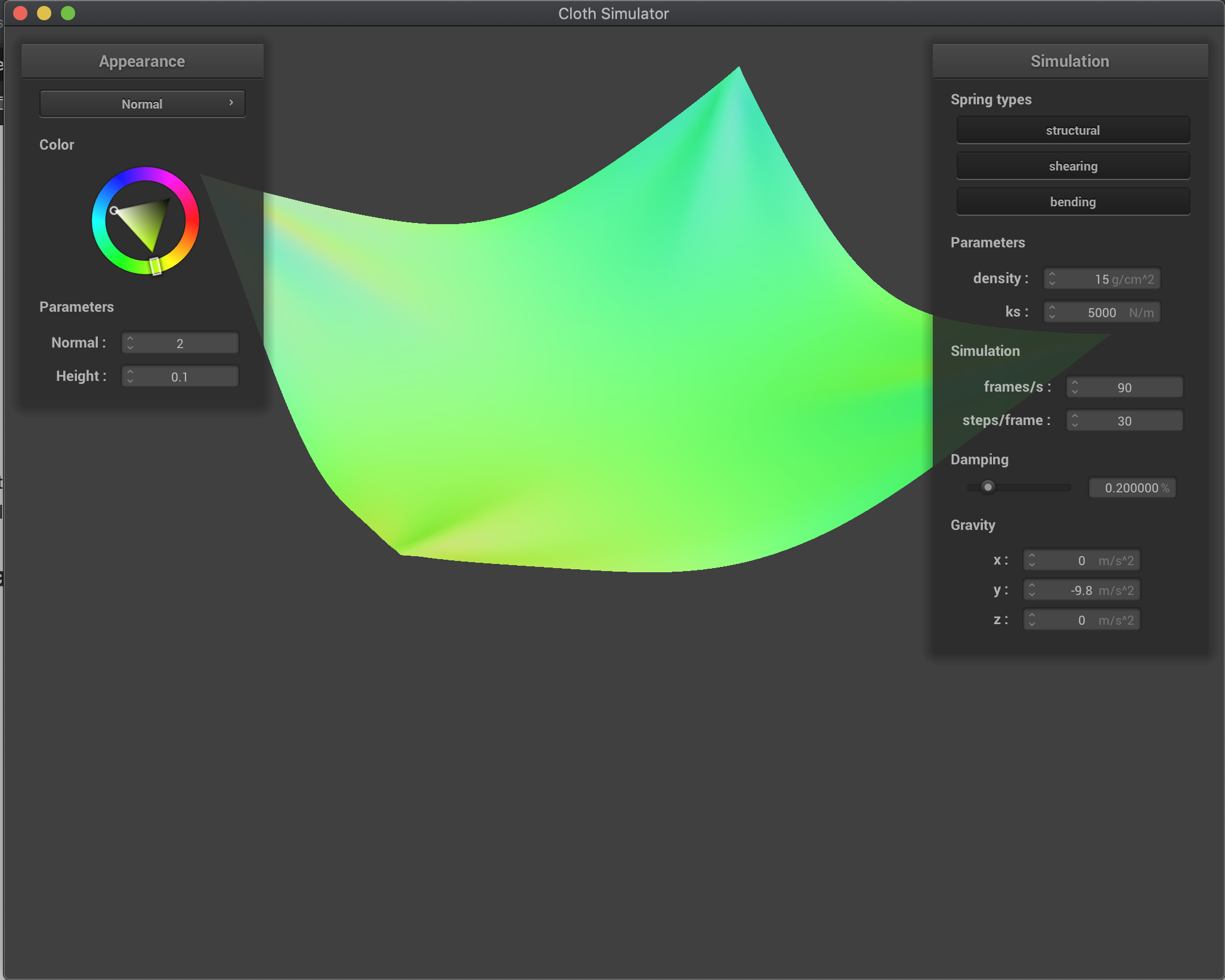
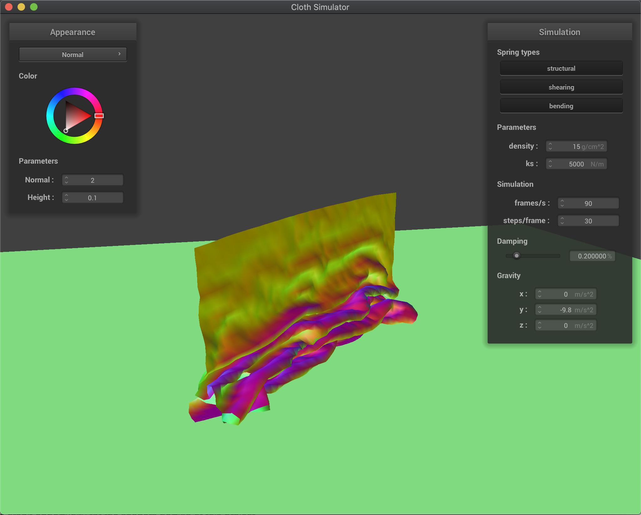
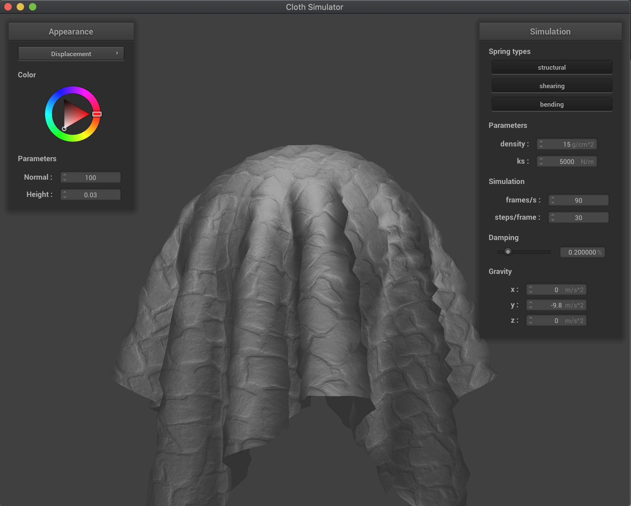
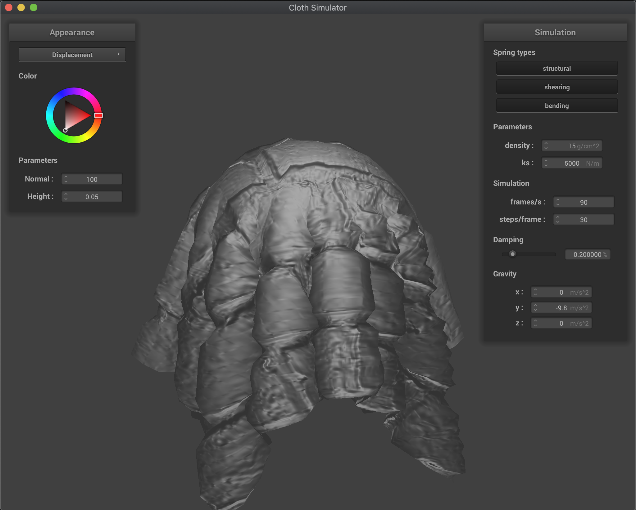
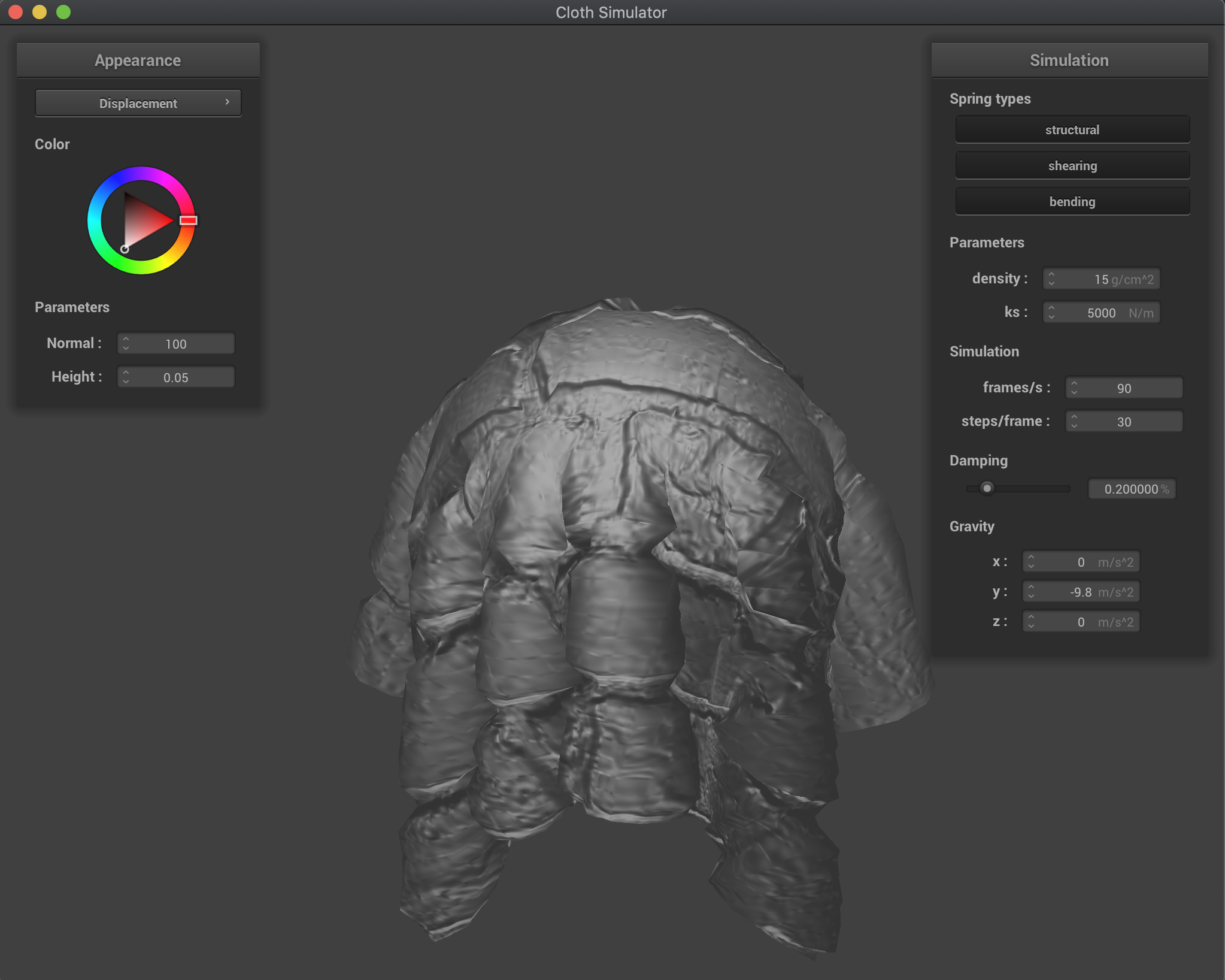
For displacement mapping, I kept the same bump mapping logic, but instead in the .vert file, I shifted the position of the vertex in the direction of the normal, scaled by the same function h(u, v) and a height scaling constant k_h. This produced the result below:

The main difference between these two techniques is that displacement mapping actually shifts the position of the vertices, whereas bump mapping does not, even though both compute the same vector normal in order to create similar effects. As can be seen, the displacement mapping is more jagged along the surface, and it has more obvious protrusions compared to bump mapping, although both have distinct effects caused by the normals.

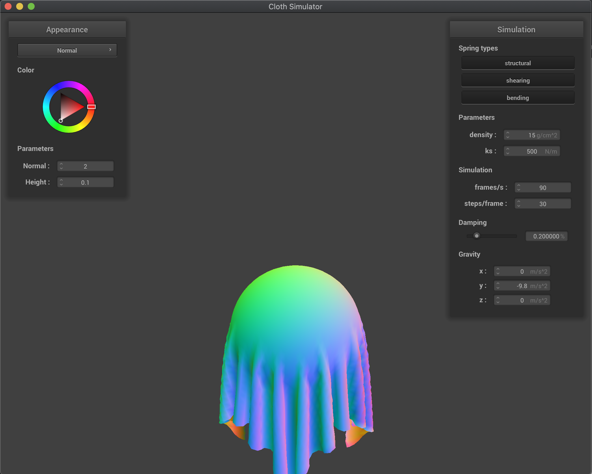
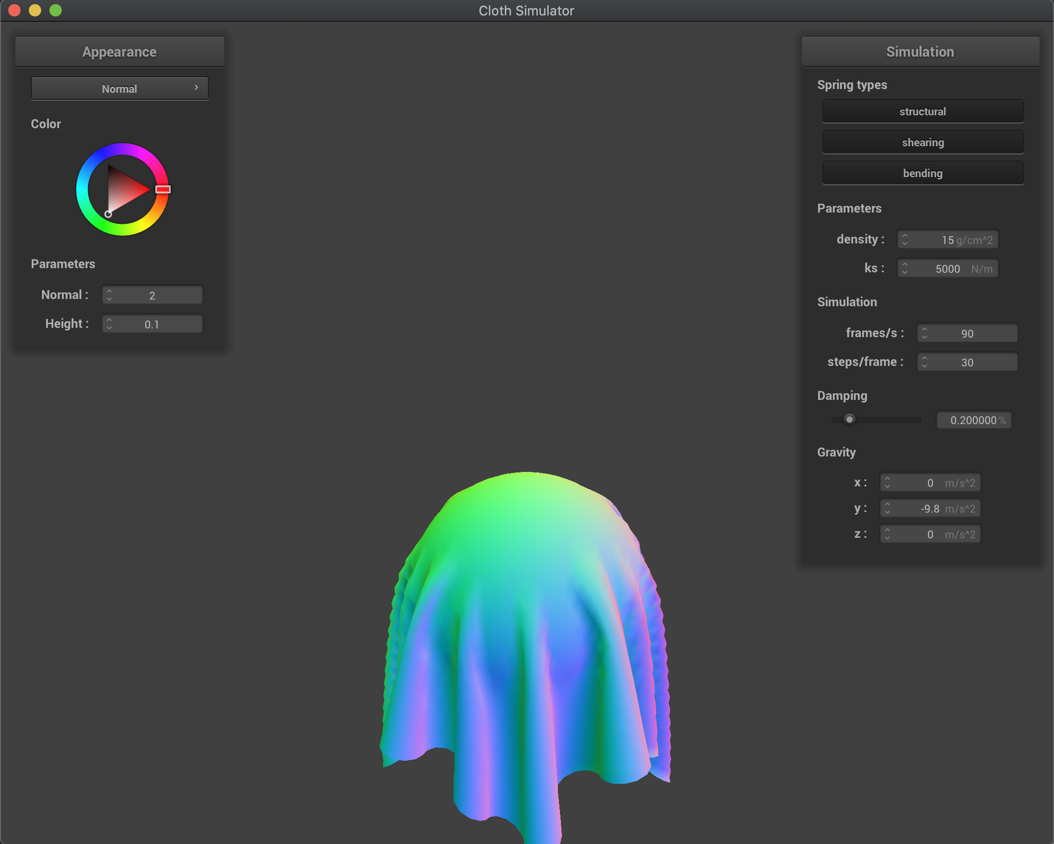
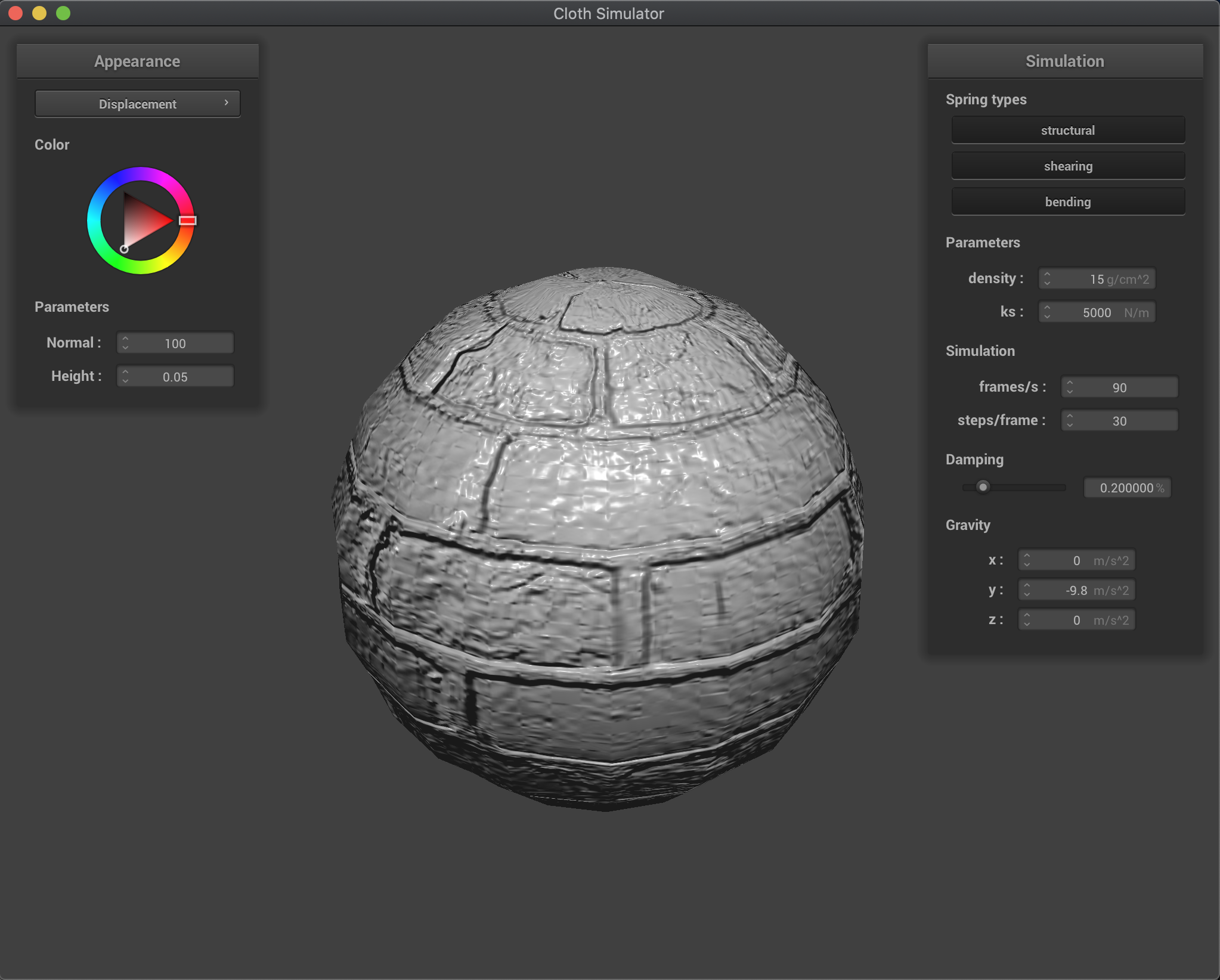
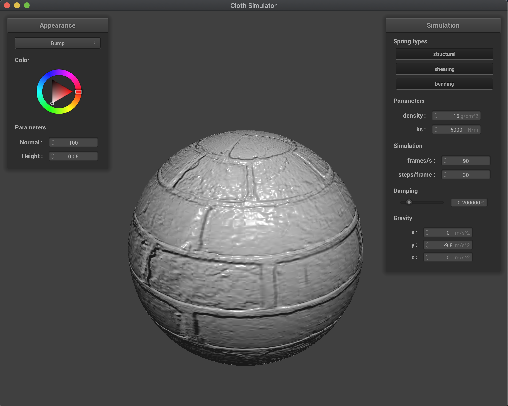
Now to experiment, I looked at the effects of both shaders with varying levels of the sphere mesh coarseness. At a resolution of 16 vertically and horizontally, note that there is not much difference between both the bump and displacement mappings. At a higher resolution of 128 however, there is a greater distinction between the two mappings, and the shifts in vertex positions in the displacement mapping are more profound. As a whole though, both create more realistic shading than previously before, and really help to make the texture chosen pop out. Note that the spheres and cloth were screenshotted with different Blinn-Phong parameters, which is the reason there is some distinction in color; however, this doesn't affect the actual mappings of the normals. Also note that the decision of which texture to use can greatly affect whether the shifts in vertex positions are more obvious, since that is determined by the normals. The default texture showed better displacement results, but this one was chosen just for the sake of selecting a different texture:

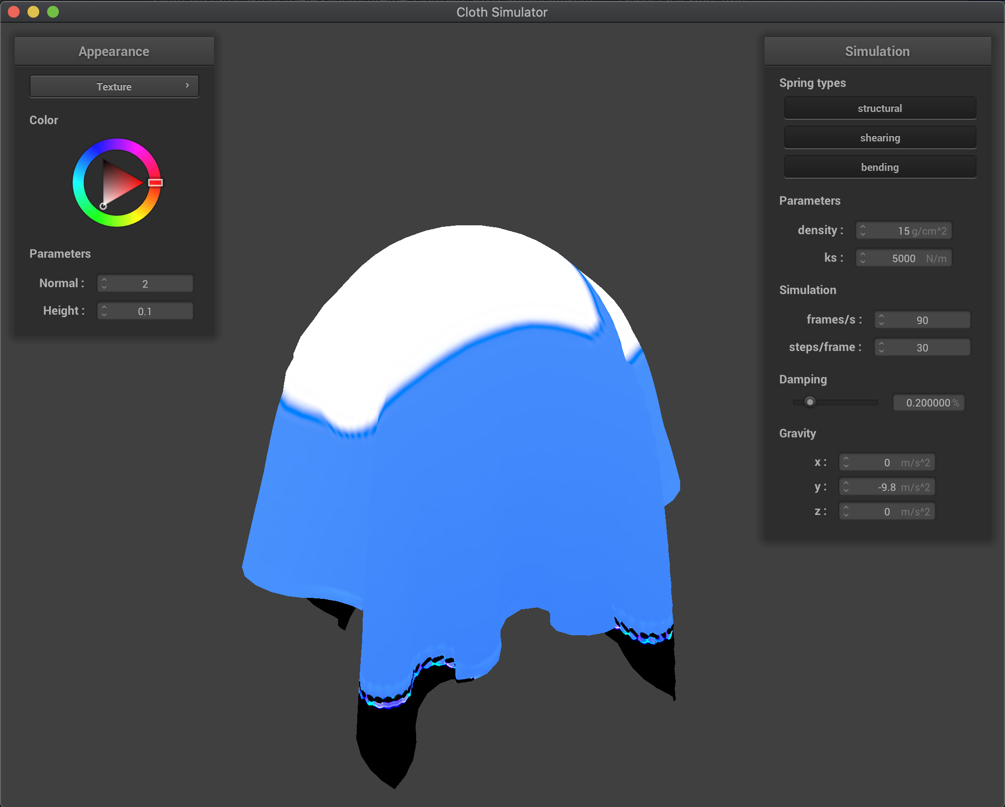
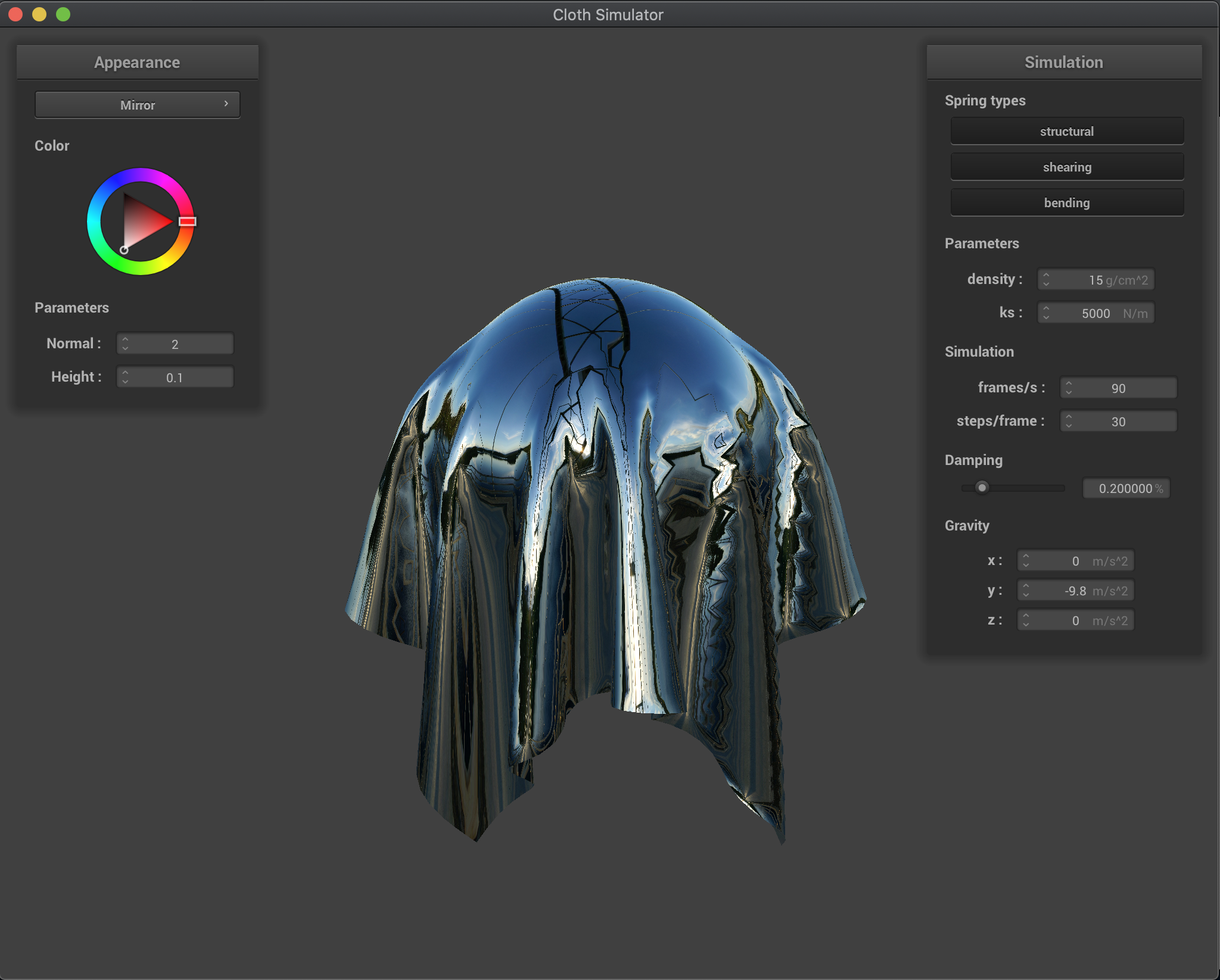
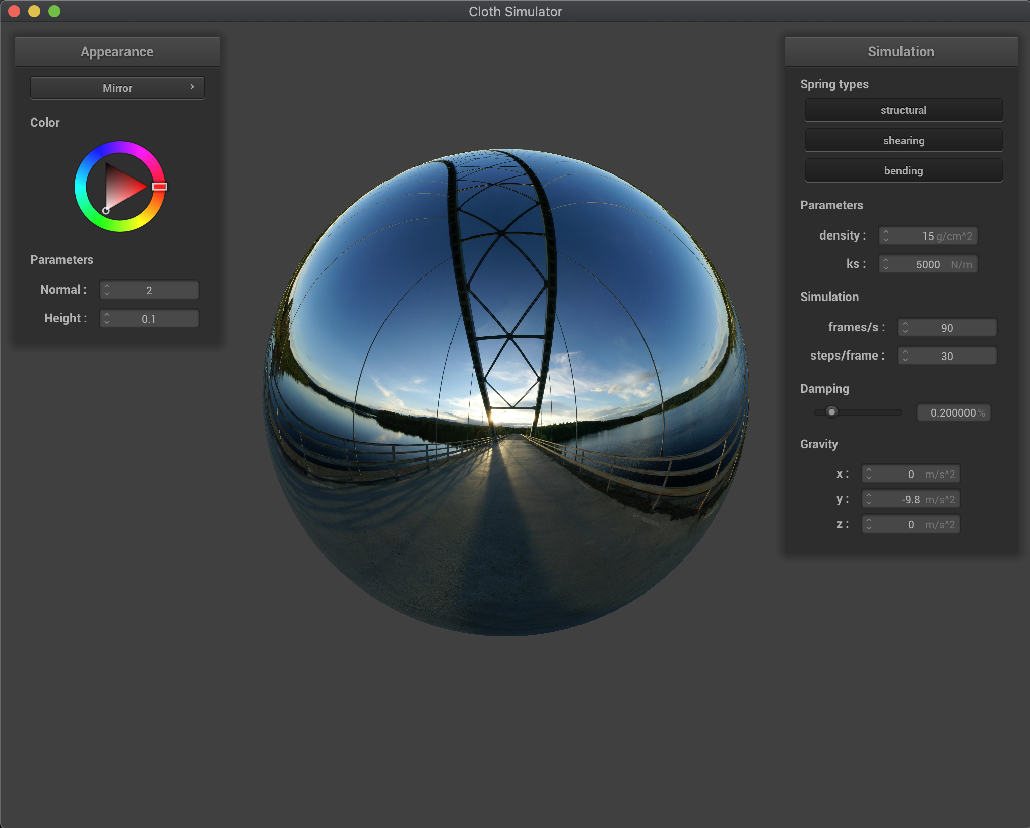
Task 5: Environment-mapped Reflections

The final shader program that I implemented was the mirror shader, that essentially sampled the environment for the reflected vector's incoming radiance. Basically, I took the input eye-ray, the vector from the vertex position to the camera, and then reflected it across the surface normal using the equation -eye_ray + 2 * (dot(eye_ray, n)) * n. I then used this reflected vector to sample from the given environment map, resulting in mirror like effects on my cloth and sphere. Below are the results: